
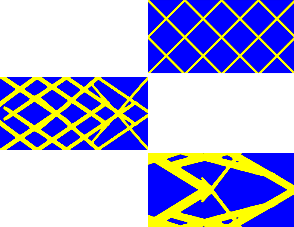
はじめに
近年、構造最適化手法の一種であるトポロジー最適化が実際の製品にも適用され始め、その応用分野は弾性体、振動、伝熱、熱流体など多岐に渡ります。
トポロジー最適化手法は、これまでの歴史の中で様々な手法が提案されてきました[1-5]。トポロジー最適化を実問題に適用する際には、製品の製造方法や扱う物理現象、目的に応じて手法を選択する必要があり、各手法への理解を深めることが重要です。
本記事では、代表的な手法である密度法、均質化法、レベルセット法、そしてここ数年盛んに研究が行われているMoving Morphable Components(MMC)の概要や特徴を紹介します。特に、MMCの解説記事は少ないため、数式表現に踏み込んで説明したいと思います。そして、密度法とMMCをMATLABで実装し、結果の違いを見ていきたいと思います。
感度解析
数理最適化には、目的関数の設計変数に関する感度(勾配)を用いる勾配法、生物の進化を模倣した進化的手法、ランダムに設計空間を探索する総当たり的手法、目的関数の形や勾配などを用いずに入力値と出力値のみから最適解を見つけるブラックボックス最適化など様々な手法が存在します。
本記事では、実装の容易さと探索効率の良さから勾配法を用います。
勾配法は、周囲が霧で見渡せない山の斜面での下山によく例えられます。現時点の設計変数\(x\)における目的関数\(f(x)\)の値と勾配\(\frac{df}{dx}\)の情報のみから、少しずつ目的関数が小さい方向へ移動することで最小値を目指します。
感度解析とは、目的関数の設計変数に関する感度(勾配)を算出し、目的関数が減少(または増加)するための設計変数を動かすべき方向を解析することを意味します。
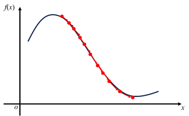
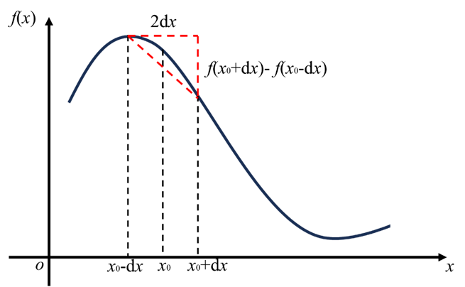
目的関数が設計変数で陽に記述されていれば直接微分により感度を算出できますが、そうでない場合は設計変数に微小値を与えて近似的に微分値を計算します。これを数値微分と呼びます。
\(\frac{df(x)}{dx}
≃\frac{f(x+dx)-f(x-dx)}{2dx}\)
後ほど実装するプログラムにおいて、密度法は目的関数が設計変数で陽に表されているため直接微分をし、MMCは目的関数が設計変数で陽に表されていないため数値微分を用います。
数値微分は目的関数によらず感度を算出できるという利点がありますが、目的関数を複数回評価する必要があるため計算コストを増大させてしまうという欠点があります。
代表的なトポロジー最適化手法の概要
均質化法に基づくトポロジー最適化
均質化法に基づくトポロジー最適化は、マイクロストラクチャと呼ばれる周期的に並ぶミクロ構造を設計領域内に定義し、そのミクロ構造を制御するパラメタを設計変数としてマクロな構造特性を最適化するというコンセプトの手法です。

解析する際には、均質化を行い、マクロ的な力学特性が実際にマイクロストラクチャを有する構造と整合するように定式化します。
手法が提案された当時、マイクロストラクチャを製造することは困難でしたが、近年はAdditive Manufacturingの発展により、様々な材料でマイクロストラクチャの製造が可能となりました。
弊社で均質化法によるトポロジー最適化を行ったラティス構造の試作モデルを掲載します。
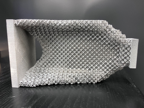
マイクロストラクチャの疎密により幾何形状を表現できていることがわかります。このように均質化法に基づくトポロジー最適化は、微細構造を用いて構造部材を最適化したい場合に用いる手法です。
均質化についてより詳しく知りたい方は、過去の技術記事をご一読ください。
(2)アディダス3DPシューズ解説:圧縮力をせん断変形に変換するメカニカルメタマテリアルの設計
密度法
密度法は、解析に用いる各有限要素に0〜1の規格化された材料濃度を設計変数として与え、その濃度の濃淡を最適化するというコンセプトの手法です。

最適化の枠組みの中で中間濃度にペナルティを与え、なるべく濃度が0と1に二分化されるように工夫します。それでも境界部等でどうしても中間濃度が発生してしまうため、最終的には閾値を設けて材料の有無を決定します。比較的自由度の高い複雑な幾何形状を表現できることが特徴で、多くの汎用CAEソフトウェアに実装されています。
一方、有限要素をピクセルとしたドット絵で幾何形状を表現することに等しく、滑らかな幾何形状を得るには多くの有限要素数を必要とするため、計算コストが増大してしまいます。
また、過度に複雑な幾何形状が創出されてしまう可能性があり、製造方法に合わせて幾何形状をデフォルメすることが必要となる場合もあります。一見、構造の意味することがわからない局所解に収束してしまうこともしばしばあり、創出される幾何形状の示唆することを読み取り、初期値を変えながら最適解を見つけなければならない場合もあります。
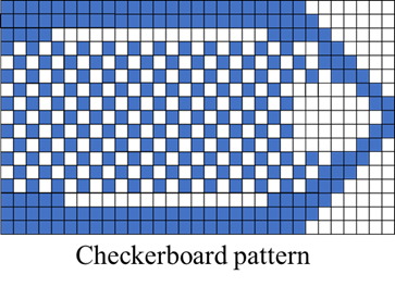
さらに、材料の有無が交互に並んでしまうチェッカーボード現象が問題の1つとして知られています。製造が困難かつ実際に製造したら格子が連結されている角部で壊れてしまいそうですが、数値解析上では剛性が高く評価されるため創出されてしまいます。対応策として、感度や密度にフィルターをかける方法が挙げられます。
レベルセット法に基づくトポロジー最適化
レベルセット法に基づくトポロジー最適化は、設計領域内に分布するレベルセット関数と呼ばれるスカラ関数を設計変数とし、レベルセット関数のゼロ等位面を材料の境界と定義し、少しずつ発展させることによって幾何形状を創出するというコンセプトの手法です。
境界の発展は、疑似的な時間を導入し、目的関数に関する感度を駆動力とすることで達成しています。
密度法のように有限要素単位のドット絵で幾何形状を表現するような手法ではなく、自由形状な境界を持つ幾何形状を明瞭に表現できることが特徴です。
実装上は、設計領域全体の有限要素節点におけるレベルセット関数値のゼロ等位面を更新することとなるため、節点の数に比例して設計変数の数が増加してしまいます。
上記3手法の理論やその応用については,文献[6,7]を始め、数多くのウェブページでも詳説されておりますのでご参照ください。
Moving Morphable Components(MMC)
Moving Morphable Components(MMC)は、解析に用いる有限要素とは別に、あらかじめ最適幾何形状の部材となり得る要素を「構成要素」として設計領域に配置しておき、構成要素の移動、回転、拡大、縮小、重ね合わせで幾何形状を表現するというコンセプトの手法です。

事前に配置する構成要素数は任意に決められるため、製造方法や設計制約に応じて創出される幾何形状の複雑さを制御することが可能です。
幾何形状の表現と解析に用いる有限要素が独立しており、密度法と比べて荒いメッシュ数でも明瞭に幾何形状を表現できます。設計変数の数は構成要素の数のみに依存しているため、有限要素の数を増やしても設計変数の数には無関係です。
加えて、構成要素の寸法を設計変数としているため、部材の寸法を最適化の枠組みの中で直接制御できるのも特徴の1つです。製造上の理由等で最大最小としたい部材寸法が決まっている場合に有用です。
一方、初期値が収束解に影響を与えてしまうため、注意して決定する必要があります。設計変数は、構成要素の中心座標、縦横寸法、回転角度の5つで,それらの初期値を調整しながら最適化を行わなければなりません。
さらに、形状の決まった構成要素の集合体で幾何形状を表現するため、伝熱問題や流路問題など複雑かつ滑らかな形状を表現すべき問題には不向きだと言えるでしょう。しかし、MMCで曲線的で自由な形状表現を可能にするという趣旨の研究は行われており[8-10]、今後、様々な問題への応用が期待できます。
MMCの構成要素を数学的に記述する方法
このような概念に基づいてトポロジー最適化をする場合、設計領域上で構成要素が存在する領域をどのように数学的に表現するのかという疑問が浮かびます。以降でこの疑問について説明していきます。
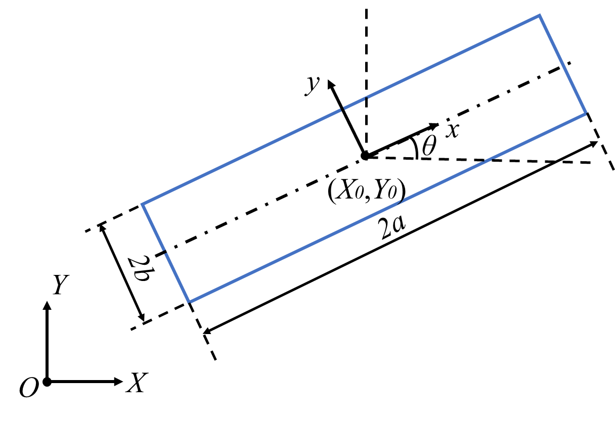
前述の通り,MMCの\(i\)番目構成要素\(d_i\)は構成要素の中心座標\((X_0,Y_0)\)、長手寸法\(L\)、短手寸法\(t\),回転角度\(θ\)の5つです。
\(\begin{align*}
        d_{i}
        =
       \left[
            \begin{array}{ccc}
                 X_{0} & Y_{0} & L& t & θ\\
            \end{array}
        \right]
    \end{align*}\)
これら5つの設計変数を用い、構成要素の有無は
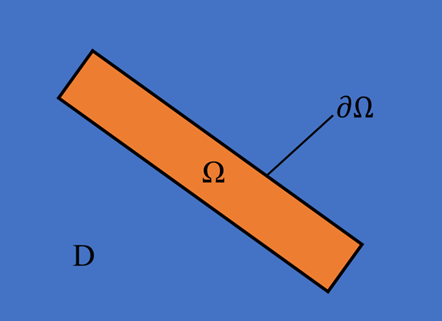
\(φ(X,Y)>0⇔(X,Y)∈Ω\)
\(φ(X,Y)=0⇔(X,Y)∈∂Ω\)
\(φ(X,Y)<0⇔(X,Y)∈D/Ω\)
ただし、
\(φ(X,Y)=1-\left(\frac{cosθ(X-X_0)+sinθ(Y-Y_0)}{L/2}\right)^m-\left(\frac{-sinθ(X-X_0)+cosθ(Y-Y_0)}{t/2}\right)^m\)
という陰関数\(φ\)で表されます。ただし、\(m\)は偶数の定数です。1行目から順に見ていきましょう。
まず、1~3行目は、\(φ\)が正の座標は構成要素が存在する領域、\(φ\)が0の座標は構成要素の境界、\(φ\)が負の座標は構成要素が存在しない領域を表すことを示しています。このように、MMCでは、構成要素の存在をトポロジー記述関数と呼ばれる陰関数\(φ\)の正負で陰的に表現します。
次に、4行目の\(φ\)が具体的に何を元としている関数なのかを説明します。
はじめに、長径が\(a\)、短径が\(b\)の楕円の方程式を考えてみます。
\(\left(\frac{x}{a}\right)^2+\left(\frac{y}{b}\right)^2=1\)
この楕円を拡張した概念に、超楕円(ラメ曲線)があります。超楕円とは,楕円の累乗部分が2以外の偶数値も取れるよう拡張した関数であり、\(m\)の値を増加させるにつれて徐々に長方形に近づいていきます。後ほど行う実装では\(m=6\)と設定しました。
\(\left(\frac{x}{a}\right)^m+\left(\frac{y}{b}\right)^m=1\)
\(⇔1-\left(\frac{x}{a}\right)^m-\left(\frac{y}{b}\right)^m=0\)
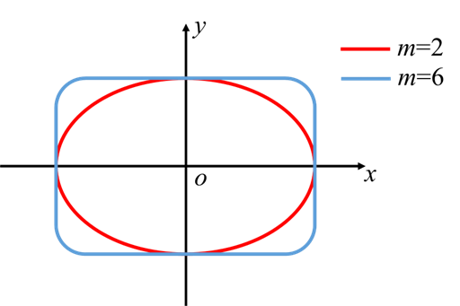
上記の超楕円の式は閉曲線を表しているため、\(x\)、\(y\)の関数とすることで、閉曲線の内側、外側、境界線を\(ψ\)の値で指し示すことが可能となります。
\(ψ(x,y)=1-\left(\frac{x}{a}\right)^m-\left(\frac{y}{b}\right)^m\)
ここで、\(ψ\)は超楕円の中心に固定された局所座標系\(x\)、\(y\)で定義された関数です。超楕円の並進・回転を実現するために、全体座標系に\(ψ\)を座標変換し、これを\(φ\)と定義します。
\(\begin{bmatrix} x \\ y \end{bmatrix}=
\begin{bmatrix}
cosθ & sinθ \\ -sinθ & cosθ
\end{bmatrix}
\begin{bmatrix}
X-X_0 \\ Y-Y_0
\end{bmatrix}=
\begin{bmatrix}
cosθ(X-X_0)+sinθ(Y-Y_0) \\ -sinθ(X-X_0)+cosθ(Y-Y_0)
\end{bmatrix}\)
\(φ(X,Y)=1-\left(\frac{cosθ(X-X_0)+sinθ(Y-Y_0)}{a}\right)^m-\left(\frac{-sinθ(X-X_0)+cosθ(Y-Y_0)}{b}\right)^m\)
以上でトポロジー記述関数を導出することができました。
後ほど実装するプログラムの解析では、トポロジー記述関数の\(X\),\(Y\)に各有限要素節点の座標を入力し、材料の有無を調べます。そして、有限要素の周囲4節点のトポロジー記述関数値から、その節点が構成する有限要素の剛性を決定し、解析を行います。
トポロジー最適化の実装
最適化問題設定
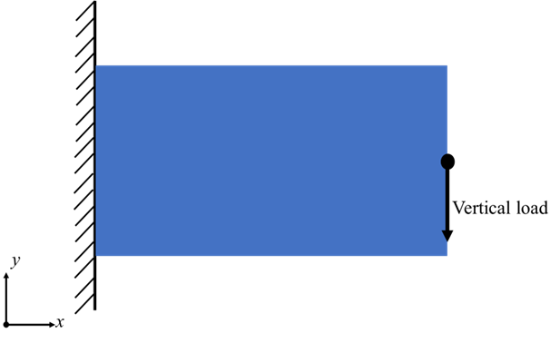
ベンチマーク問題として、以下のような問題設定でトポロジー最適化を行いました。
・境界条件:片持ち
・荷重条件:自由端中央に垂直荷重
・目的:平均コンプライアンス最小化
・制約条件:設計領域の40 %体積制約
なお、最適化の繰り返し計算は収束状況に関わらず200回目まで行いました。
密度法による最適化結果
密度法による初期幾何形状、最適化後の幾何形状を示します。
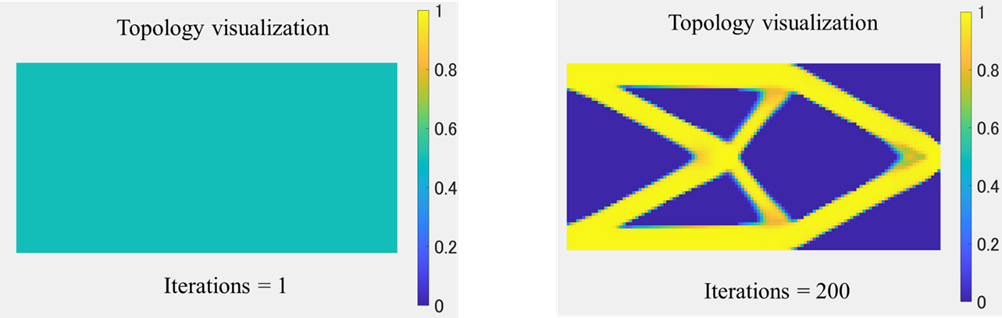
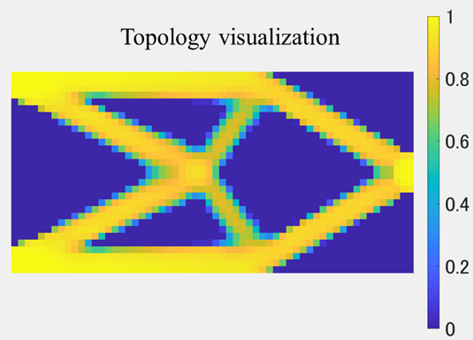
120×60と要素分割数を細かく設定したため、明瞭に幾何形状を表現できています。試しに要素分割数を60×30にしてみましょう。幾何形状の解像度が粗くなっていることを確認できます。
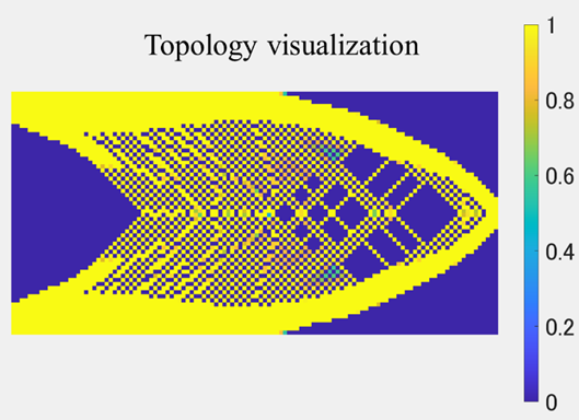
また、感度へのフィルタリングを行わない場合も試してみましょう。要素の有無が交互に並ぶチェッカーボード現象を確認できます。
MMCによる最適化結果
MMCによる最適幾何形状と各構成要素を見やすくするために構成要素の塗りつぶしを無くした図を示します。なお、構成要素の数や初期配置については様々な決定方法が考えられますが、今回は先行研究に倣い、なるべく構成要素が設計領域内で均等に配置されるよう、16個の構成要素を斜めに交差させ敷き詰めました。
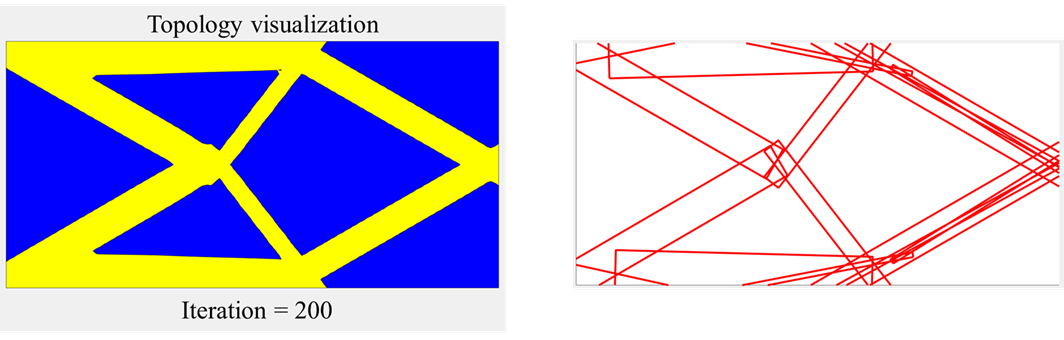
どのように最適幾何形状が創出されたのかを確認するために最適化Iterationが1、10、30のときの結果を示します。

このように、各構成要素が徐々に最適幾何形状に適合していることがわかります。
前述の通り、幾何形状の表現が有限要素の数から独立しているので、メッシュをある程度荒くしても幾何形状の創出に影響はありません。これを確認すべく、有限要素数を60×30としたときの結果も見てみましょう。
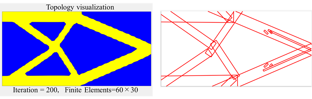
このように、メッシュを荒くしても同傾向の幾何形状を明瞭に表現可能なことが確認できました。
次に、創出された幾何形状と計算コストの観点から両手法の結果を比較したいと思います。
創出された幾何形状の比較
両手法で創出された幾何形状を比較します。
密度法により創出された幾何形状は表現に制限が無いため、滑らかに幾何形状を表現できています。
一方で、MMCは長方形の構成要素の集合で幾何形状を表現するため、構造的特徴は密度法による結果と一致しているものの、洗練されていない幾何形状になっていることがわかります。
具体的には、構成要素同士の連結部分の不連続さや、構造上不要と思われる突起が表れてしまっていることが挙げられます。
理由としては、構成要素同士の連続性に何の拘束も課されていないこと、構成要素の変化は目的関数の感度にのみ依存しており、図に示す突起のように微小な部分は感度へ与える影響も微小で、最適化の中で修正すべき部分として感知されないことが考えられます。
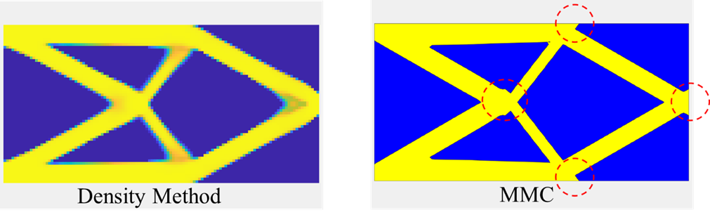
今回解いたShort beamのベンチマーク問題で得られる幾何形状はそのほとんどが直線形状で構成されていましたが、最適幾何形状がより複雑な曲線形状を含んでいる問題の場合、密度法とMMCの幾何形状表現の差がより顕著に表れるでしょう。
計算コストの比較
有限要素数が120×60、60×30のときの密度法とMMCの計算コストについて、有限要素数、設計変数の数、計算時間、各計算時間の割合を表にまとめます。
密度法の設計変数の数は有限要素数と同じ7200個と1800個、MMCは構成要素数を16個としたため、設計変数の数は有限要素数によらず80個です。MATLABの時間計測機能により、最適化Iterationが200回終わるまでの計算時間を計測しました。
| Method | Finite elements | Design variables | Time [s] | Ratio [%] |
|---|---|---|---|---|
| Density method | 120×60 | 7200 | 293.2 | 100 |
| Density method | 60×30 | 1800 | 59.2 | 20.2 |
| MMC | 120×60 | 80 | 31.3 | 10.7 |
| MMC | 60×30 | 80 | 13.9 | 4.7 |
表の通り、計算時間は密度法とMMCで比較すると大きな差があることがわかりました。
先ほどお見せした、創出される幾何形状の解像度が低い60×30の密度法でも、120×60のMMCよりも約2倍計算コストがかかるとわかります。
このように、幾何形状の表現自由度の観点では密度法が、計算コストの観点ではMMCが優れていることがわかり、一概にどちらが優れていると言えるわけではありません。
例えば、製造制約から単純な幾何形状を創出したい場合や、最適幾何形状のおおよその傾向を確認したい場合はMMCのような簡易的手法が良く、複雑な幾何形状の特徴を詳細に把握したい場合には密度法のようなフルサイズのトポロジー最適化が適しているでしょう。
おわりに
本記事では、密度法、均質化法、レベルセット法、MMCの4つのトポロジー最適化手法について特徴を紹介し、密度法とMMCを実装した結果を比較しました。両者とも長所と短所があり、製造方法や扱う物理現象、設計制約によって使い分ける必要があることを説明しました。
今回はトポロジー最適化手法自体に焦点を当てて説明をしましたが、実問題に適用する際に最も重要なことは、
・設計対象をどのようにモデル化し、いかに最適化として解ける問題に落とし込むか
・最適化結果を人間がどのように解釈し、いかに製品として形にするか
です。
実問題においては、モデル化や使用する最適化手法によっては無意味な幾何形状が創出されることもしばしばあります。また、トポロジー最適化結果をそのまま設計結果とすることは現状難しく、コンピュータと人間が連携しながら製品として形にすることが必要となります。
弊社の強みはまさにここにあり、モデル化や手法の選択、結果を解釈し形にすることにおいて様々な知見やノウハウを保有しています。例として、トポロジー最適化を用いて設計を行っている技術記事を是非ご一読ください。
本記事では構造強度に関する単純なベンチマーク問題を扱いましたが、実問題にいくつかのトポロジー最適化を適用した際の結果の差異についてもいつか紹介したいと思います。
皆さんもトポロジー最適化をご自身で実装し、各手法の仕組みや結果を比べてみてください。新たな発見があり、理解が深まることと思います。
参考
[1] Bendsøe, M. P., and Kikuchi, N., “Generating Optimal Topologies in Structural Design Using a Homogenization Method,” Computer Methods in Applied Mechanics and Engineering, Vol. 71, No. 2, 1988, pp. 197–224.
[2] Dorn, W., Gomory, R. and Greenberg, H., “Automatic Design of Optimal Structures,” Journal de Mecanique, Vol. 3, No. 6, 1964, pp. 25–52.
[3] Bendsøe, M. P., “Optimal Shape Design as a Material Distribution Problem,” Structural Optimization, Vol. 1, No. 4, 1989, pp. 193–202.
[4] Sethian, J. A., and Wiegmann, A., “Structural Boundary Design via Levelset and Immersed Interface Methods,” Journal of Computational Physics, Vol. 163, No. 2, 2000, pp. 489–528.
[5] Guo, X., Zhang, W. S., and Zhong, W. L., “Doing Topology Optimization Explicitly and Geometrically-A New Moving Morphable Components Based Framework,” Journal of Applied Mechanics, Vol. 81, No. 8, 2014, p. 081009.
[6] 日本計算工学会 編,「トポロジー最適化」,丸善出版,2013.
[7] 近藤 継男,矢地 謙太郎,西脇 眞二 共著,「トポロジー最適化の基礎 弾性体ならびに熱流体工学諸問題への応用のために」,コロナ社,2024.
[8] Zhang, Z., Yuan, J., Zhang, J., and Guo, X., “A New Topology Optimization Approach based on Moving Morphable Components (MMC) and the Ersatz Material Model,” Structural and Multidisciplinary Optimization, Vol. 53, No. 6, 2016, pp. 1243–1260.
[9] Guo, X., Zhang, W., Zhang, J., and Yuan, J., “Explicit Structural Topology Optimization Based on Moving Morphable Components (MMC) with Curved Skeletons,” Computer Methods in Applied Mechanics and Engineering, Vol. 310, 2016, pp. 711–748.
[10] Otsuka, K., Dong, S., Kuzuno, R., Sugiyama, H., Makihara, K., “Moving Morphable Multi Components Introducing Intent of Designer in Topology Optimization,” AIAA Journal, Vol. 61, No. 4, pp. 1720–1734.
Introduction
In recent years, a type of structural optimization method called topology optimization has begun to be applied to actual products, with applications spanning a wide range of fields such as elasticity, vibration, heat transfer, and thermal fluid dynamics.
Topology optimization methods have been proposed in various forms through its history [1-5]. When applying topology optimization to practical problems, it is important to choose the appropriate method based on the manufacturing method of the product, the physical phenomena involved, and the objectives, the consideration of which require a deep understanding of each method.
This article introduces an overview of representative methods including homogenization method, density method, level set method, and Moving Morphable Components (MMC), which has been actively researched in recent years. Particularly, as there are few explanatory articles on MMC, we would like to delve into the mathematical expressions. Additionally, we will implement the density method and MMC in MATLAB to observe the differences in results.
Sensitivity Analysis
In mathematical optimization, various methods exist, including gradient-based methods that utilize sensitivity with respect to the design variables, evolutionary methods inspired by biological evolution, exhaustive methods that randomly explore the design space, and black-box optimization that finds optimal solutions solely based on input-output pairs without utilizing the form or gradients of the objective function.
In this article, we will utilize gradient-based methods due to their ease of implementation and efficient exploration. Gradient-based methods utilize sensitivity with respect to the design variables, often likened to descending a mist-covered slope on a mountain. By using information about the value of the objective function \(f(x)\) and its gradient \(\frac{df}{dx}\) at the current design variable \(x\), the method gradually moves towards directions where the objective function decreases, aiming to find the minimum value.
Sensitivity analysis means calculating the sensitivity (gradient) of the objective function with respect to the design variables and analyzing how the objective function behaves when the design variables change.
If the objective function is explicitly described in terms of the design variables, sensitivity can be directly calculated through differentiation. If not, sensitivity is approximated by providing a small value to the design variables, which is known as numerical differentiation.
\(\frac{df(x)}{dx}
≃\frac{f(x+dx)-f(x-dx)}{2dx}\)
In the program implemented later, the density method uses direct differentiation because the objective function is explicitly represented by the design variables, while MMC uses numerical differentiation because the objective function is not explicitly represented by the design variables.
Numerical differentiation has the advantage of being able to calculate sensitivity independently of the objective function, but it has the disadvantage of increasing computational cost due to the need to evaluate the objective function multiple times.
Overview of typical topology optimization methods
Topology Optimization Based on Homogenization Method
Topology optimization based on the homogenization method is a technique that defines periodically arranged microstructures within the design domain and optimizes macrostructural properties by controlling parameters that govern these microstructures as design variables.
The calculation is formulated so that the mechanical properties of the homogenized structure match those of the actual structure with microstructure.
At the time when the method was proposed, manufacturing microstructures was challenging. However, recent advancements in Additive Manufacturing have made it possible to manufacture microstructures using various materials.
Here, we present a prototype model of lattice structure obtained through topology optimization based on the homogenization method.
It can be observed that the topology is represented by the sparsity of the microstructure. Topology optimization based on the homogenization method is used when optimizing structural components using fine structures.
For those who want to learn more about homogenization, please refer to our past technical articles.
Homogenizing Mechanical Metamaterial
(1) Homogenization of lattice structure
(2) Homogenization of lattice structure
Density Method
Density method is a technique where normalized material densities ranging from 0 to 1 are assigned as design variables to each finite element used in the analysis, with the concept of optimizing the distribution of these densities.
Within the optimization framework, penalties are applied to intermediate densities to encourage a binary distribution closer to 0 and 1. Nonetheless, intermediate densities may still occur, particularly at boundary regions, so a threshold is eventually set to determine the presence or absence of material. This method has capability to represent relatively complex topologies with high degrees of freedom and is implemented in many general-purpose CAE software.
However, akin to representing topology with pixelated artwork where each finite element serves as a pixel, obtaining smooth topology requires a large number of finite elements, leading to increased computational costs.
In addition, overly complex topologies may be created, and topologies may need to be deformed to fit the manufacturing methods. It is not uncommon for solutions to converge to local optima that are initially unintelligible structurally, requiring interpretation of the topology and iterative refinement of the initial values to find the optimal solution.
Additionally, the checkerboard pattern phenomenon, where material presence alternates, poses a known challenge. Although such patterns may seem structurally weak, they are often evaluated as having high rigidity in numerical analysis. Filtering sensitivity or density is one approach to mitigate this issue.
Topology Optimization Based on Level Set Method
Topology optimization based on the level set method employs a scalar function called the level set function as the design variable, distributed within the design domain. The zero level set of this function defines the material boundary, evolving gradually to generate topology.
Boundary evolution introduces a pseudo-time concept, driving sensitivity with respect to the objective function.
Unlike methods such as the density method that represent topology with finite element unit pixelation, this method allows for clear representation of topologies with free-form boundaries.
In actual implementation, the boundaries of the level set function are updated at every finite element node throughout the design domain, so the number of design variables increases in proportion to the number of nodes.
For further details on the theory and applications of these three methods, please refer to references [6,7], as well as numerous web resources available.
Moving Morphable Components (MMC)
Moving Morphable Components (MMC) is a method based on the concept of representing topology through the movement, rotation, enlargement, reduction, and superposition of predefined elements called "constituent elements," which are placed in the design space separately from the finite elements used in the analysis.
The number of constituent elements placed as initial condition can be arbitrarily determined, allowing control over the complexity of the topology generated according to manufacturing methods and design constraints.
The representation of topology and the finite elements used for analysis are independent, allowing for clear representation of topology even with a coarse mesh compared to density methods. The number of design variables depends only on the number of constituent elements, regardless of the number of finite elements.
Furthermore, since the dimensions of the constituent elements are treated as design variables, it is possible to directly control the dimensions of the members within the framework of optimization. This is useful when there are constraints on the minimum or maximum dimensions of members for manufacturing reasons.
However, it is important to note that the initial values can influence the converged solution. Design variables consist of the center coordinates, longitudinal and transverse dimensions, and rotation angle of the constituent elements, and optimization must be performed repeatedly adjusting their initial values.
Additionally, since MMC represents topology using a set of predefined elements with determined shapes, it may not be suitable for problems requiring representation of complex and smooth shapes, such as heat transfer or flow path problems. However, research aiming to enable MMC to represent curved and freeform shapes is underway, and various applications to different problems can be expected in the future.
Mathematical Description of MMC Constituent Elements
Based on this concept, one may wonder how to mathematically represent the regions where constituent elements exist in the design space. Let's explain this question below.
As mentioned earlier, the \(i\)th constituent element \(d_i\) consists of five design variables: the center coordinates \((X_0, Y_0)\), the longitudinal dimension \(L\), the transverse dimension \(t\), and the rotation angle \(θ\).
\(\begin{align*}
        d_{i}
        =
       \left[
            \begin{array}{ccc}
                 X_{0} & Y_{0} & L& t & θ\\
            \end{array}
        \right]
    \end{align*}\)
Using these five design variables, the existence of constituent elements can be determined by the implicit function \(φ\), which is defined as:
\(φ(X,Y)>0⇔(X,Y)∈Ω\)
\(φ(X,Y)=0⇔(X,Y)∈∂Ω\)
\(φ(X,Y)<0⇔(X,Y)∈D/Ω\)
Where,
\(φ(X,Y)=1-\left(\frac{cosθ(X-X_0)+sinθ(Y-Y_0)}{L/2}\right)^m-\left(\frac{-sinθ(X-X_0)+cosθ(Y-Y_0)}{t/2}\right)^m\)
\(m\) is an even constant. Now, let's break down the equation line by line.
First, lines 1 to 3 indicate that positive values of \(φ\) represent regions where constituent elements exist, \(φ = 0\) represents the boundaries of constituent elements, and negative values of \(φ\) represent regions where constituent elements do not exist. Thus, in MMC, the existence of constituent elements is implicitly expressed by the positive and negative values of the implicit function \(φ\).
Next, line 4 describes what specific function \(φ\) is based on.
First, let's consider the equation of an ellipse with major axis \(a\) and minor axis \(b\):
\(\left(\frac{x}{a}\right)^2+\left(\frac{y}{b}\right)^2=1\)
An extension of this ellipse concept is the hyperellipse (lame curve). A hyperellipse is a function that extends the power part of an ellipse to take even values other than 2, gradually approaching a rectangle as the value of \(m\) is increased. In the calculation perfoemed later, we set \(m=6\).
\(\left(\frac{x}{a}\right)^m+\left(\frac{y}{b}\right)^m=1\)
\(⇔1-\left(\frac{x}{a}\right)^m-\left(\frac{y}{b}\right)^m=0\)
The equation of this superellipse represents a closed curve, so by treating \(x\) and \(y\) as functions, it is possible to use the value of \(ψ\) to indicate the inside, outside, and boundary of the closed curve.
\(ψ(x,y)=1-\left(\frac{x}{a}\right)^m-\left(\frac{y}{b}\right)^m\)
Here, \(ψ\) is a function defined in the local coordinate system \(x\) and \(y\) fixed at the center of the hyperellipse. To translate and rotate the hyperellipse, we transform \(ψ\) to a global coordinate system of coordinates, which we define as \(φ\).
\(\begin{bmatrix} x \\ y \end{bmatrix}=
\begin{bmatrix}
cosθ & sinθ \\ -sinθ & cosθ
\end{bmatrix}
\begin{bmatrix}
X-X_0 \\ Y-Y_0
\end{bmatrix}=
\begin{bmatrix}
cosθ(X-X_0)+sinθ(Y-Y_0) \\ -sinθ(X-X_0)+cosθ(Y-Y_0)
\end{bmatrix}\)
We have now derived the topology description function.
In the subsequent calculations, we input the coordinates of each finite element node into the \(X\) and \(Y\) of the implicit function \(φ\), and examine the presence of constituent elements. Then, based on the \(φ\) values of the four nodes surrounding each finite element, we determine the rigidity of the finite element composed by those nodes and perform the analysis.
Topology optimization implementation
Optimization Problem Setup
As a benchmark, topology optimization was solved with the following problem setup:
- Boundary conditions: Cantilever
- Load conditions: Vertical load at the center of the free end
- Objective: Minimization of strain energy
- Constraint: 40% volume constraint of the design domain
The optimization iterations were conducted up to the 200th iteration regardless of convergence status.
Optimization Results by Density Method
The initial and optimized topologies by the density method are shown below.
The fine mesh with 120 × 60 elements allows for a clearer representation of topology.
Let's try reducing the element divisions to 60×30. As a result, we can observe a decrease in the resolution of the topology representation.
Furthermore, let's explore the results without sensitivity filtering. We can observe the checkerboard pattern in which elements are arranged alternately.
Optimization Results by MMC
The optimized topology by MMC is shown below, where the fill of constituent elements is removed for better visibility. For this case, 16 constituent elements were placed diagonally to evenly cover the design domainas the initial condition, following previous research methodologies.
To understand how the optimized topology was generated, results at iteration 1, 10, and 30 are shown below.
It's evident that each constituent element gradually conforms to the optimized topology over iterations.
As mentioned earlier, since MMC's topology representation is independent of the number of finite elements, the topology can be clearly represented even with a coarse mesh. Let's examine the results with a mesh of 60×30 elements.
It's evident that similar topology trends can be clearly represented even with a coarser mesh, validating the independence of topology representation from the number of mesh divisions.
Next, let's compare the results of both methods from the perspectives of the generated topology and computational cost.
Comparison of Generated Topology
We'll compare the topologies generated by both methods. While the density method can represent topologies without restrictions, allowing for smooth topology representations, MMC, which represents topology using a collection of rectangular constituent elements, yields less refined topologies. Although structural features are consistent between the results of the density method and MMC, the MMC topology appears less refined, exhibiting discontinuities in the connections between constituent elements and unnecessary protrusions.
The lack of constraints on the continuity between constituent elements and the dependency of constituent element variations solely on sensitivity may contribute to such differences. Minute features like the protrusions shown in the figure may have minimal effects on sensitivity, thus not being recognized as areas needing modification during optimization.
Although both methods produced similar shapes because the benchmark problem solved in this article mainly consisted of linear shapes, if the optimization problem involves more complex curved shapes, the disparity in topology representations between the density method and MMC would be more pronounced.
Comparison of Computational Costs
Let's compare the computational costs of the density method and MMC for mesh sizes of 120×60 and 60×30 elements. Following table summarizes the optimization method, the number of finite elements, design variables, and required computation time. Relative differences in computation time from the density method for 120×60 elements are also shown.
| Method | Finite elements | Design variables | Time [s] | Ratio [%] |
|---|---|---|---|---|
| Density method | 120×60 | 7200 | 293.2 | 100 |
| Density method | 60×30 | 1800 | 59.2 | 20.2 |
| MMC | 120×60 | 80 | 31.3 | 10.7 |
| MMC | 60×30 | 80 | 13.9 | 4.7 |
The number of design variables for the density method corresponds to the number of finite elements, i.e., 7200 and 1800 for mesh sizes of 120×60 and 60×30, respectively. For MMC, the number of design variables remains constant at 80, regardless of the number of finite elements. MATLAB's timing feature was used to measure the computation time until the 200th iteration of optimization.
As shown in the table, there is a significant difference in computation time between the density method and MMC. Even for the density method with a lower resolution of 60×30 elements, it required approximately twice the computational cost of MMC with a mesh size of 120×60.
Thus, while the density method offers greater freedom in topology representation, MMC excels in terms of computational cost. It's essential to consider these aspects when choosing between the two methods.
For example, if simple topologies are desired due to manufacturing constraints or to obtain a rough idea of the optimized topology, MMC or similar simplified methods may be suitable. Conversely, for detailed understanding of complex topology features, the density method or full-size topology optimization may be preferable.
Conclusion
In this article, we introduced four topology optimization methods: homogenization method, density method, level set method, and MMC, highlighting their characteristics. We then compared the results of optimization by the density method and MMC, both of which we implemented. Each method has its strengths and weaknesses, and the choice between them depends on manufacturing methods, physical phenomena, and design constraints.
We focused on explaining topology optimization methods in this article. However, when applying these methods to real-world problems, the most critical factors include:
- How to model the design object and formulate it as an optimization problem
- How to interpret the optimization results and shape them into tangible products
In real-world applications, meaningless topologies may be generated depending on the modeling and method selection. Moreover, directly using topology optimization results as design outcomes remains challenging. Thus, collaboration between computers and humans is necessary to shape the optimized topology into tangible products.
Our strength lies precisely in this area, as we possess various knowledge and expertise in modeling, method selection, interpretation of results, and product shaping. Please feel free to explore our technical articles on topology optimization:
Heat Sink Design Case Study by Thermal Fluid Topology Optimization
Design Example : Lower Arm for Automobile
Although we addressed a simple benchmark problem related to structural strength in this article, we would like to introduce the differences in optimization results when applying various topology optimizations to real-world problems someday.
We encourage you to implement topology optimization methods yourself and compare the results. It will lead to new discoveries and deepen your understanding of the subject.
Reference
[1] Bendsøe, M. P., and Kikuchi, N., “Generating Optimal Topologies in Structural Design Using a Homogenization Method,” Computer Methods in Applied Mechanics and Engineering, Vol. 71, No. 2, 1988, pp. 197–224.
[2] Dorn, W., Gomory, R., and Greenberg, H., “Automatic Design of Optimal Structures,” Journal de Mecanique, Vol. 3, No. 6, 1964, pp. 25–52.
[3] Bendsøe, M. P., “Optimal Shape Design as a Material Distribution Problem,” Structural Optimization, Vol. 1, No. 4, 1989, pp. 193–202.
[4] Sethian, J. A., and Wiegmann, A., “Structural Boundary Design via Levelset and Immersed Interface Methods,” Journal of Computational Physics, Vol. 163, No. 2, 2000,
pp. 489–528.
[5] Guo, X., Zhang, W. S., and Zhong, W. L., “Doing Topology Optimization Explicitly and Geometrically-A New Moving Morphable Components Based Framework,” Journal of Applied Mechanics, Vol. 81, No. 8, 2014, p. 081009.
[6] 日本計算工学会 編,「トポロジー最適化」,丸善出版,2013.
[7] 近藤 継男, 矢地 謙太郎, 西脇 眞二 共著,「トポロジー最適化の基礎 弾性体ならびに熱流体工学諸問題への応用のために」,コロナ社,2024.
[8] Zhang, Z., Yuan, J., Zhang, J., and Guo, X., “A New Topology Optimization Approach based on Moving Morphable Components (MMC) and the Ersatz Material Model,” Structural and Multidisciplinary Optimization, Vol. 53, No. 6, 2016, pp. 1243–1260.
[9] Guo, X., Zhang, W., Zhang, J., and Yuan, J., “Explicit Structural Topology Optimization Based on Moving Morphable Components (MMC) with Curved Skeletons,” Computer Methods in Applied Mechanics and Engineering, Vol. 310, 2016, pp. 711–748.
[10] Otsuka, K., Dong, S., Kuzuno, R., Sugiyama, H., Makihara, K., “Moving Morphable Multi Components Introducing Intent of Designer in Topology Optimization,” AIAA Journal, Vol. 61, No. 4, pp. 1720–1734.
