
概要
本技術ブログで、均質化の話題が何度か出ておりました。
(2)アディダス3DPシューズ解説:圧縮力をせん断変形に変換するメカニカルメタマテリアルの設計
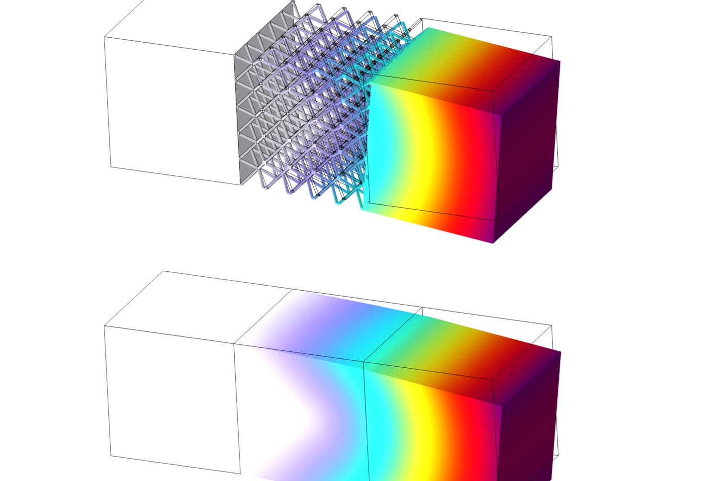
本記事では弾性体と流体(流路)の観点で、数値実験によるラティス構造の均質化方法と結果の可視化について紹介します。
本記事は前編で、弾性体の均質化について紹介します。
後編はこちら:(2)ラティス構造の均質化
なお、本記事ではAdditive Manufacturing前提となるようなラティスの均質化を紹介しておりますが、
クライアントワークにおいては、メタマテリアル構造設計技術を活用しつつ顧客の製造設備で量産可能な設計開発の支援を行うことが一般的です。
数値実験によるラティス構造の弾性行列への均質化
ラティス構造の微小変形時のふるまいを、弾性行列に入れ込む均質化手法があります。
ラティス構造相当の弾性行列を得るために、数値実験によるアプローチがよく使われます。
この数値実験の一例を紹介します。
フックの法則により、ひずみ\(\epsilon_{ij}\)と応力\(\epsilon_{k\ell}\)を紐づける行列として弾性行列\(C\)が書かれます。
\(\begin{align*}
        C
        =
       \left(
            \begin{array}{ccc}
                 c_{xxxx} & c_{xxyy} & c_{xxzz} & c_{xxyz} & c_{xxzx} & c_{xxxy}\\
                 c_{yyxx} & c_{yyyy} & c_{yyzz} & c_{yyyz} & c_{yyzx} & c_{yyxy}\\
                 c_{zzxx} & c_{zzyy} & c_{zzzz} & c_{zzyz} & c_{zzzx} & c_{zzxy}\\
                 c_{yzxx} & c_{yzyy} & c_{yzzz} & c_{yzyz} & c_{yzzx} & c_{yzxy}\\
                 c_{zxxx} & c_{zxyy} & c_{zxzz} & c_{zxyz} & c_{zxzx} & c_{zxxy}\\
                 c_{xyxx} & c_{xyyy} & c_{xyzz} & c_{xyyz} & c_{xyzx} & c_{xyxy}
            \end{array}
        \right)
    \end{align*}\)
\(\begin{align*}
        \left(
            \begin{array}{ccc}
                 \sigma_{xx} \\ \sigma_{yy} \\ \sigma_{zz} \\ \sigma_{yz} \\ \sigma_{zx} \\ \sigma_{xy}
            \end{array}
        \right)
        =
       \left(
            \begin{array}{ccc}
                 c_{xxxx} & c_{xxyy} & c_{xxzz} & c_{xxyz} & c_{xxzx} & c_{xxxy}\\
                 c_{yyxx} & c_{yyyy} & c_{yyzz} & c_{yyyz} & c_{yyzx} & c_{yyxy}\\
                 c_{zzxx} & c_{zzyy} & c_{zzzz} & c_{zzyz} & c_{zzzx} & c_{zzxy}\\
                 c_{yzxx} & c_{yzyy} & c_{yzzz} & c_{yzyz} & c_{yzzx} & c_{yzxy}\\
                 c_{zxxx} & c_{zxyy} & c_{zxzz} & c_{zxyz} & c_{zxzx} & c_{zxxy}\\
                 c_{xyxx} & c_{xyyy} & c_{xyzz} & c_{xyyz} & c_{xyzx} & c_{xyxy}
            \end{array}
        \right)
       \left(
            \begin{array}{ccc}
                 \epsilon_{xx} \\ \epsilon_{yy} \\ \epsilon_{zz} \\ 2\epsilon_{yz} \\ 2\epsilon_{zx} \\ 2\epsilon_{xy}
            \end{array}
        \right)
    \end{align*}\)
この弾性行列\(C\)は本来材料ごとに定義されますが、ラティス構造のユニットサイズより十分大きいマクロなスケールで見ればラティス構造自体を均質な材料とみなすことができるという考えのもと、ラティス構造の弾性変形時のふるまいを弾性行列\(C\)に入れ込みます。
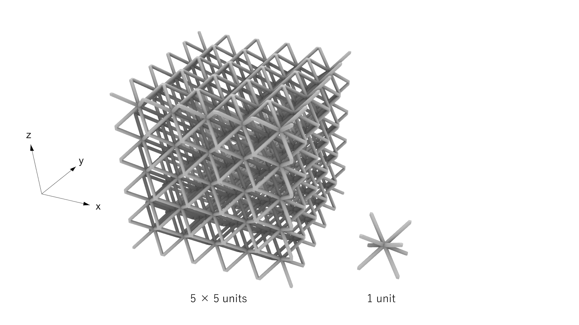
ラティス構造を均質化した弾性行列\(C\)を求めるために、ラティス構造の単位構造を取り出して数値実験を行います。
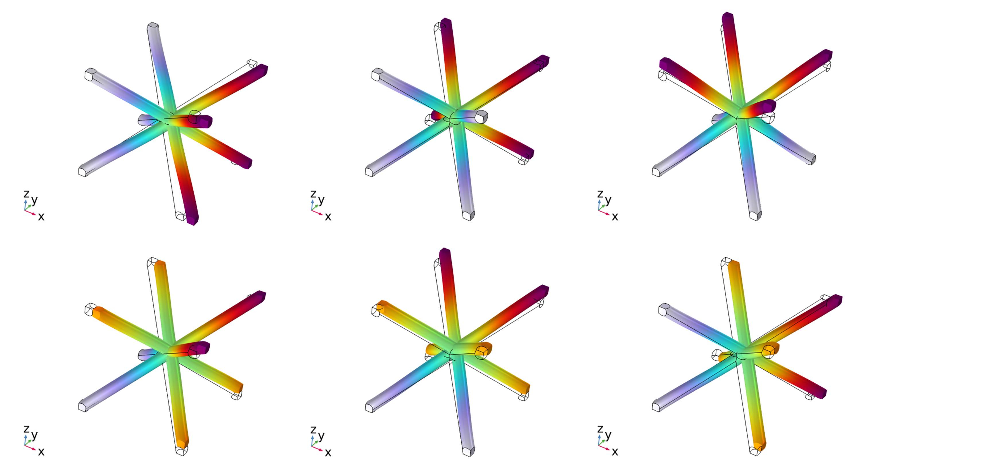
単位構造の境界面で応力とひずみの周期境界を設定したうえで、以下のように6種のひずみを与え解析を行います。
\(    \begin{align*}
       \left(
            \begin{array}{ccc}
                 \epsilon_{xx} \\ \epsilon_{yy} \\ \epsilon_{zz} \\ 2\epsilon_{yz} \\ 2\epsilon_{zx} \\ 2\epsilon_{xy}
            \end{array}
        \right)
=
       \left(
            \begin{array}{ccc}
                 1 \\ 0\\  0\\ 0 \\ 0 \\ 0
            \end{array}
        \right)
,
       \left(
            \begin{array}{ccc}
                 0 \\ 1\\  0\\ 0 \\ 0 \\ 0
            \end{array}
        \right)
,
       \left(
            \begin{array}{ccc}
                 0 \\ 0\\  1\\ 0 \\ 0 \\ 0
            \end{array}
        \right)
,
       \left(
            \begin{array}{ccc}
                 0 \\ 0\\  0\\ 1 \\ 0 \\ 0
            \end{array}
        \right)
,
       \left(
            \begin{array}{ccc}
                 0 \\ 0\\  0\\ 0 \\ 1 \\ 0
            \end{array}
        \right)
,
       \left(
            \begin{array}{ccc}
                 0 \\ 0\\  0\\ 0 \\ 0 \\ 1
            \end{array}
        \right)
    \end{align*}\)
6種のひずみの解析に対して、ボイド部分の空間も含めて各方向の平均応力\(\bar{\sigma}^{(n)}_{i,j}\)を算出します。
算出した平均応力\(\bar{\sigma}^{(n)}_{i,j}\)をもとに仮の弾性行列が以下のように得られます。
\(\begin{align*}
        \left(
            \begin{array}{ccc}
                 \sigma_{xx} \\ \sigma_{yy} \\ \sigma_{zz} \\ \sigma_{yz} \\ \sigma_{zx} \\ \sigma_{xy}
            \end{array}
        \right)
        =
       \left(
            \begin{array}{ccc}
                 \bar{\sigma}^{(1)}_{xx} & \bar{\sigma}^{(2)}_{xx} & \bar{\sigma}^{(3)}_{xx} & \bar{\sigma}^{(4)}_{xx} & \bar{\sigma}^{(5)}_{xx} & \bar{\sigma}^{(6)}_{xx}\\
\bar{\sigma}^{(1)}_{yy} & \bar{\sigma}^{(2)}_{yy} & \bar{\sigma}^{(3)}_{yy} & \bar{\sigma}^{(4)}_{yy} & \bar{\sigma}^{(5)}_{yy} & \bar{\sigma}^{(6)}_{yy}\\
\bar{\sigma}^{(1)}_{zz} & \bar{\sigma}^{(2)}_{zz} & \bar{\sigma}^{(3)}_{zz} & \bar{\sigma}^{(4)}_{zz} & \bar{\sigma}^{(5)}_{zz} & \bar{\sigma}^{(6)}_{zz}\\
\bar{\sigma}^{(1)}_{yz} & \bar{\sigma}^{(2)}_{yz} & \bar{\sigma}^{(3)}_{yz} & \bar{\sigma}^{(4)}_{yz} & \bar{\sigma}^{(5)}_{yz} & \bar{\sigma}^{(6)}_{yz}\\
\bar{\sigma}^{(1)}_{zx} & \bar{\sigma}^{(2)}_{zx} & \bar{\sigma}^{(3)}_{zx} & \bar{\sigma}^{(4)}_{zx} & \bar{\sigma}^{(5)}_{zx} & \bar{\sigma}^{(6)}_{zx}\\
\bar{\sigma}^{(1)}_{xy} & \bar{\sigma}^{(2)}_{xy} & \bar{\sigma}^{(3)}_{xy} & \bar{\sigma}^{(4)}_{xy} & \bar{\sigma}^{(5)}_{xy} & \bar{\sigma}^{(6)}_{xy}\\
            \end{array}
        \right)
       \left(
            \begin{array}{ccc}
                 \epsilon_{xx} \\ \epsilon_{yy} \\ \epsilon_{zz} \\ 2\epsilon_{yz} \\ 2\epsilon_{zx} \\ 2\epsilon_{xy}
            \end{array}
        \right)
    \end{align*}\)
弾性行列は対称行列である必要があります。また構造の対称性から値が0となるべき要素があっても数値誤差により0となりません。
対称要素の平均をとるなどの補正を加えたうえで、均質化した弾性行列を算出します。
上に図示した梁からなるラティスにおいて、ヤング率\(7×10^{10}\)Pa、ポアソン比\(0.33\)の材料において実際に均質化した弾性行列が以下になります。
\(\begin{align*}
       \left(
            \begin{array}{ccc}
                 4.89×10^8 & 4.73×10^8 & 4.73×10^8 & 0 & 0 & 0\\
                 4.73×10^8 & 4.89×10^8 & 4.73×10^8 & 0 & 0 & 0\\
                 4.73×10^8 & 4.73×10^8 & 4.89×10^8 & 0 & 0 & 0\\
                 0 & 0 & 0 & 4.41×10^8 & 0 & 0\\
                 0 & 0 & 0 & 0 & 4.41×10^8 & 0\\
                 0 & 0 & 0 & 0 & 0 & 4.41×10^8\\
            \end{array}
        \right)
    \end{align*}\)
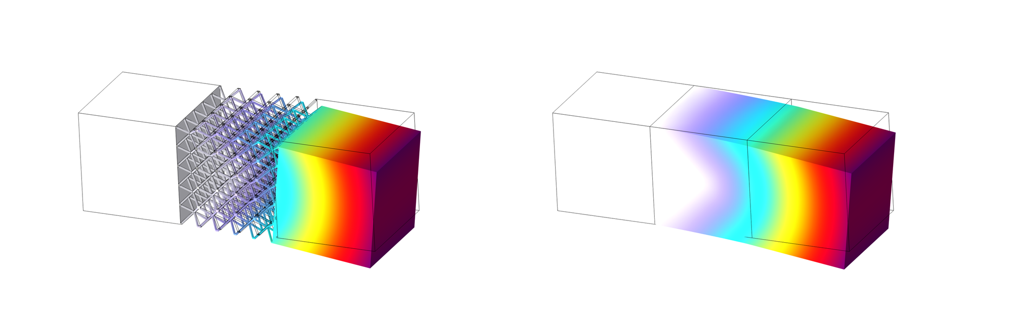
この弾性行列を用いて、\(5×5\)のラティス構造を有する片持ち梁のラティス構造部分を均質化し解析したものが以下になります。(均質化なし・ありの結果で、境界条件および可視化の変位スケーリングを合わせています。)
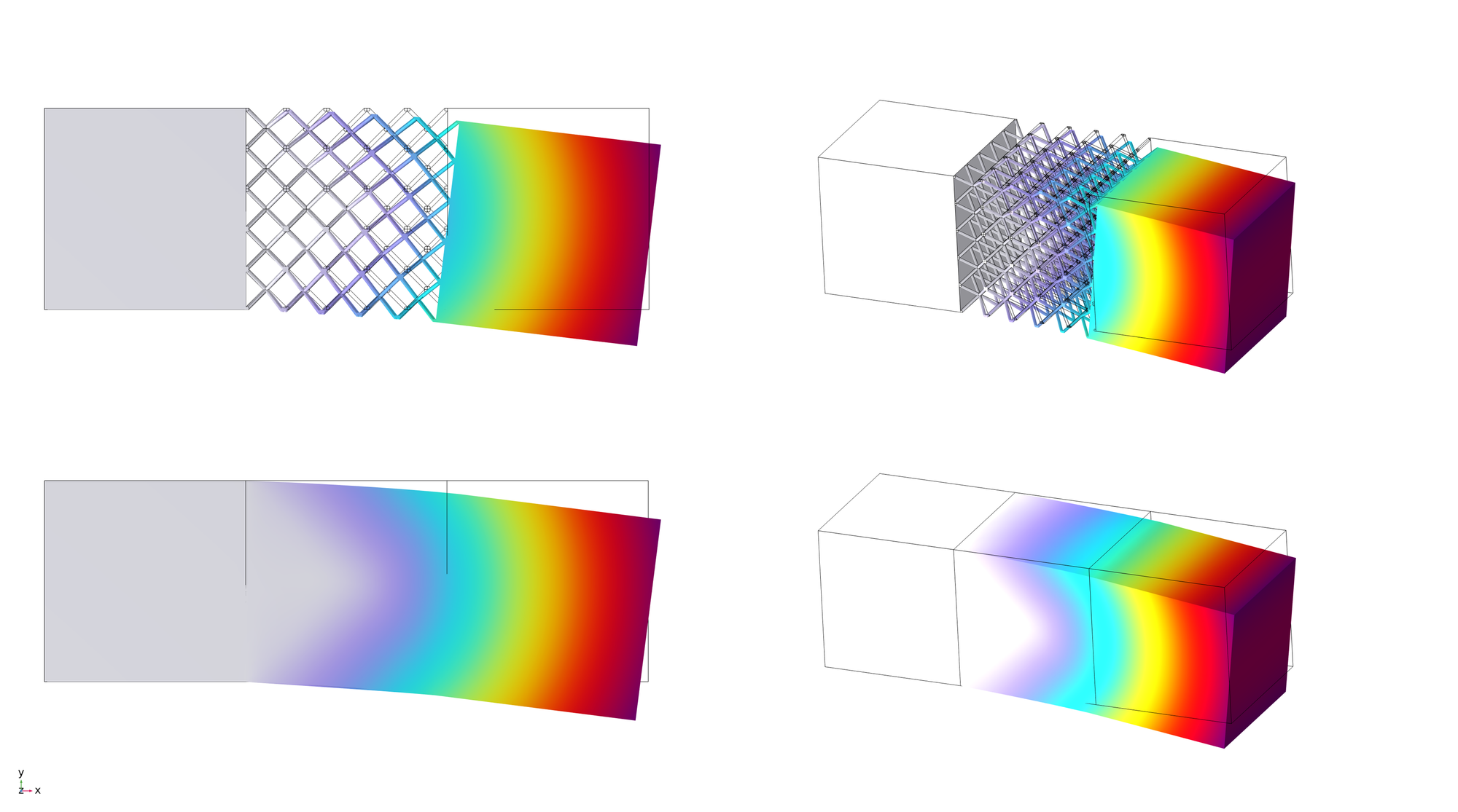
マクロな変形をよく再現できていることがわかります。
一方、フォン・ミーゼス応力をプロットすると以下のようになり、均質化によりミクロな応力は単純には見積れなくなっていることがわかります。
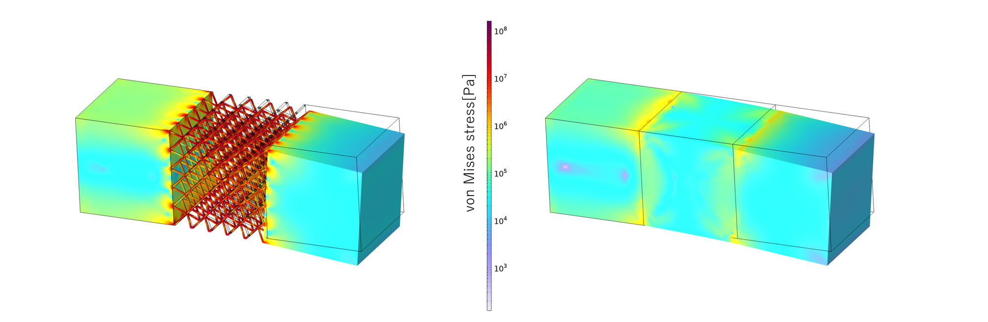
均質化による解析と合わせて局所化解析を実施することでミクロな応力もある程度見積もることができます。
また、ラティス構造の単位構造が十分に多く繰り返されている状況を仮定して均質化をしているため、繰り返し回数が少ない場合は均質化が成り立たなくなることに注意が必要です。
特徴を十分に理解したうえで、均質化を利用しましょう。
弾性行列の可視化
次に均質化した弾性行列の可視化方法を紹介します。
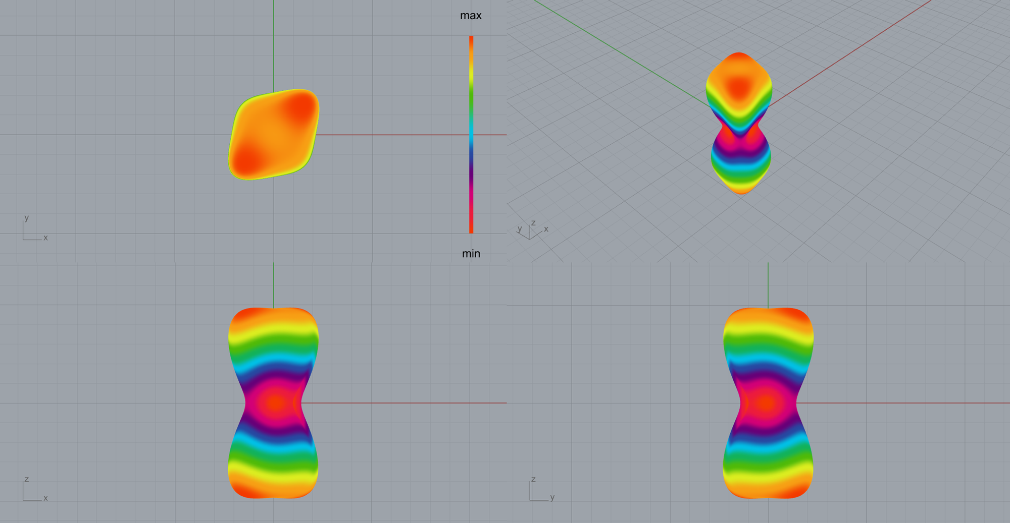
弾性行列のすべての情報を可視化するのは難しいため、ここでは各方向の有効的にはたらくヤング率の可視化を考えます。
下図のように、各方向の有効的なヤング率を、2次元または3次元の空間上で原点からそれぞれの方向にヤング率に対応する距離だけ離れた点で表現します。
それらの点を結んで線または面にすることで、各方向の有効的なヤング率を可視化します。
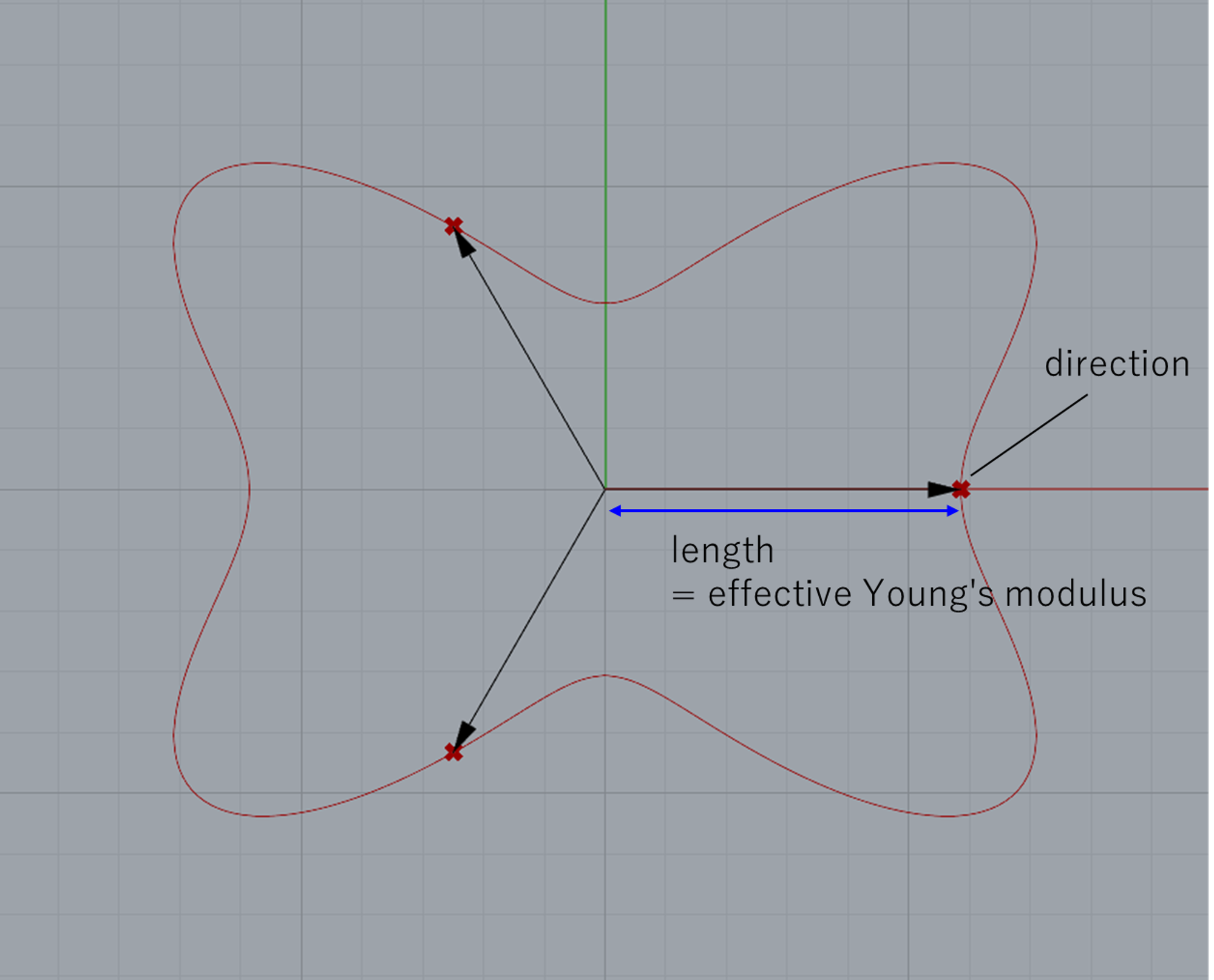
有効的なヤング率はコンプライアンス行列\(S\)(弾性行列\(C\)の逆行列)の各方向に関する対角成分(\(S_{xx},S_{yy},S_{zz}\))の逆数で定義しています。
\(x,y,z\)以外の方向に関しては、座標変換に応じて弾性行列も変換をして算出します。
この値は等方性材料においてはヤング率そのものになります。
以下で等方性材料および直行異方性材料、いくつかのラティス構造での弾性行列(ヤング率)の可視化を紹介します。
等方性材料
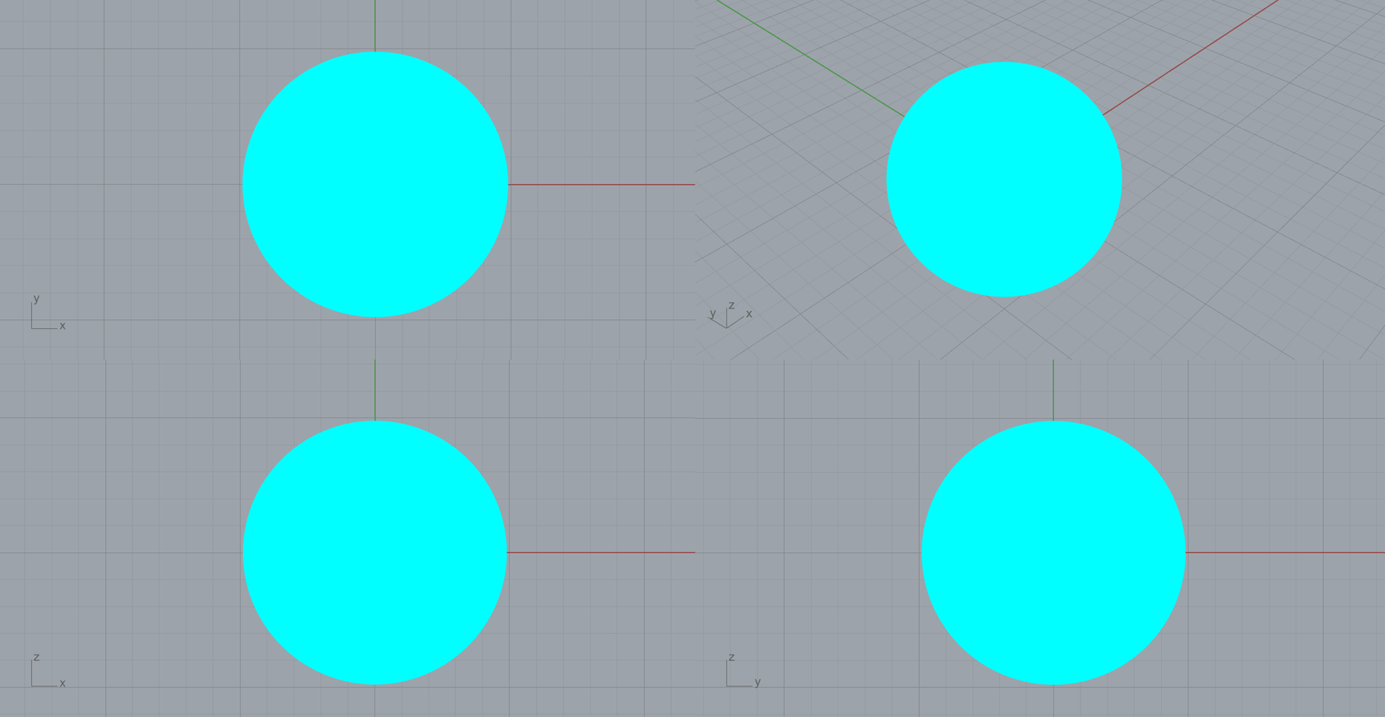
等方性材料では、当然ながら全方向でヤング率が同じとなり、3次元で可視化すると球となります。
直交異方性材料
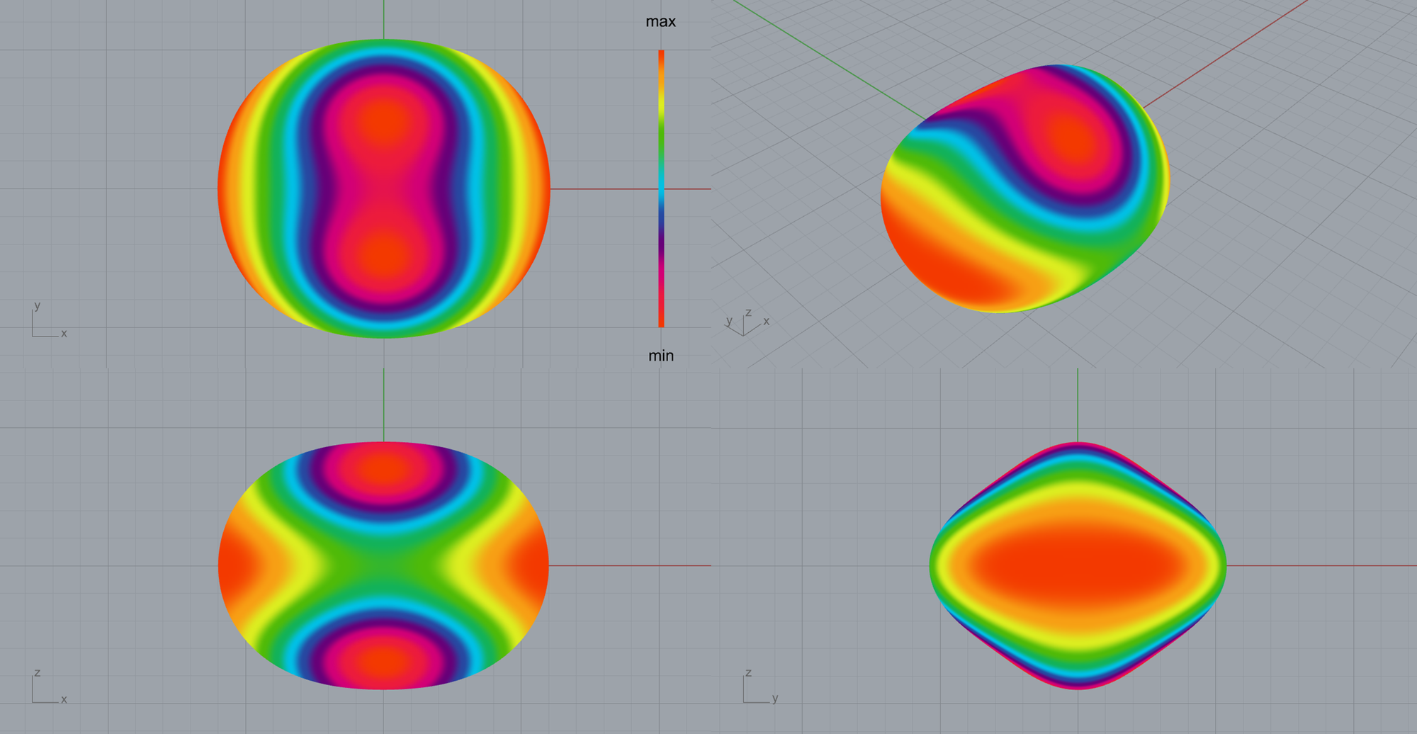
直交異方性材料(\(E_x, E_y, E_z=20, 18, 15\rm{GPa}\)、\(\nu_{xy}, \nu_{xy}, \nu_{xz}=0.12,0.10,0.14\) 、\(G_{xy}, G_{xy}, G_{xz}=9, 8, 6\rm{GPa}\)とした)では、各方向で異なる有効的なヤング率が出ていることがわかります。
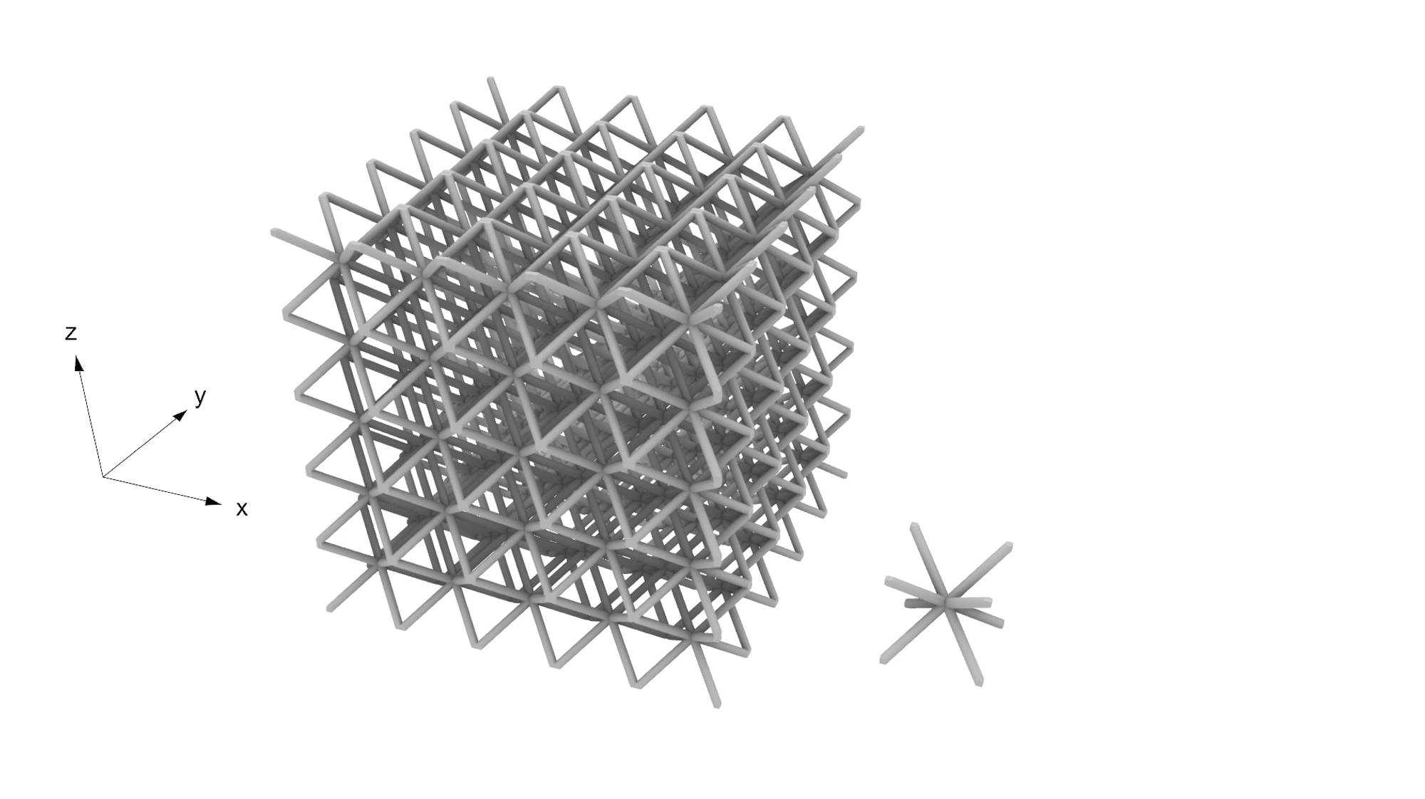
ラティス1
このラティス構造には梁が一直線に並ぶ方向があり、その方向でヤング率が大きくなっていると推察できます。
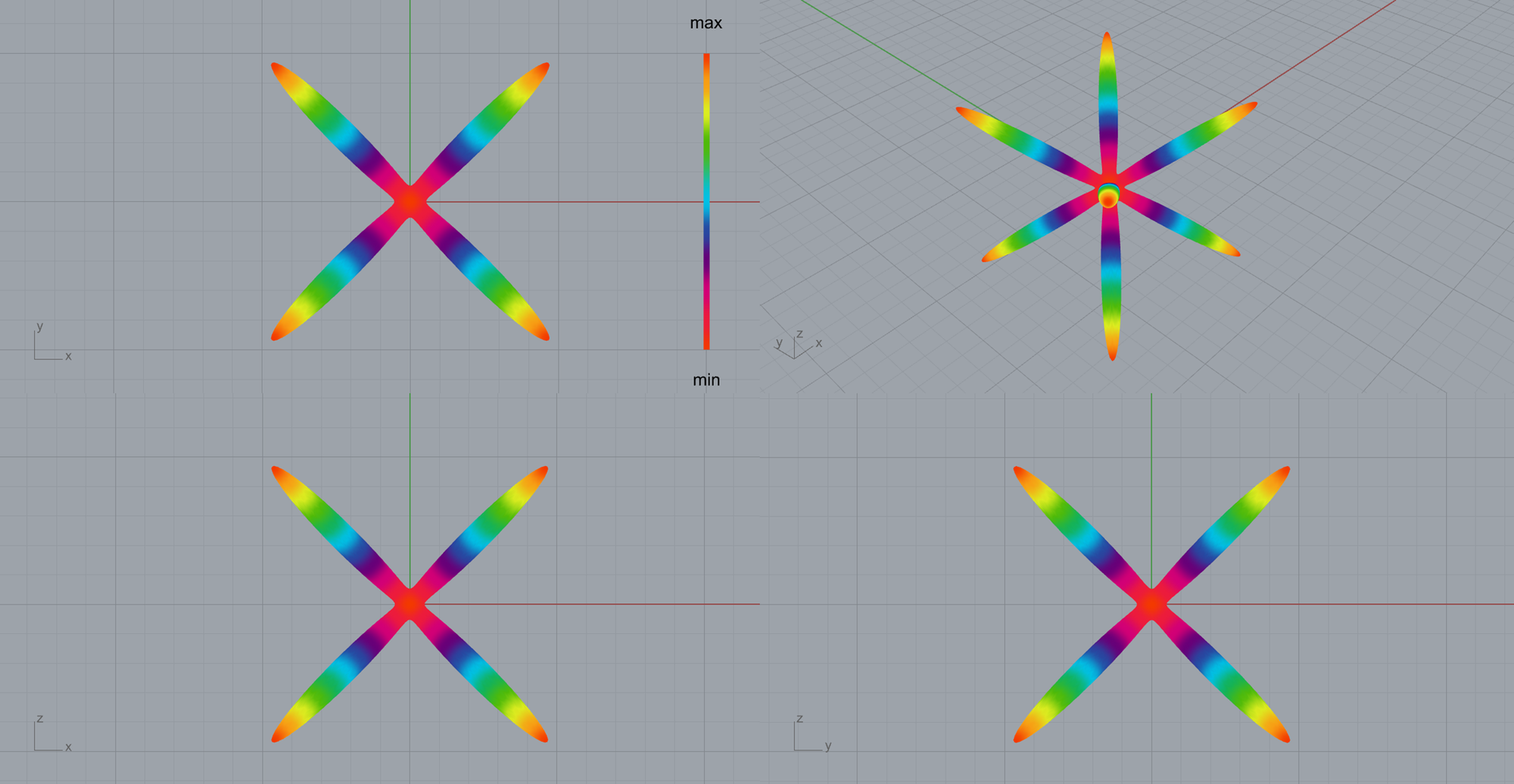
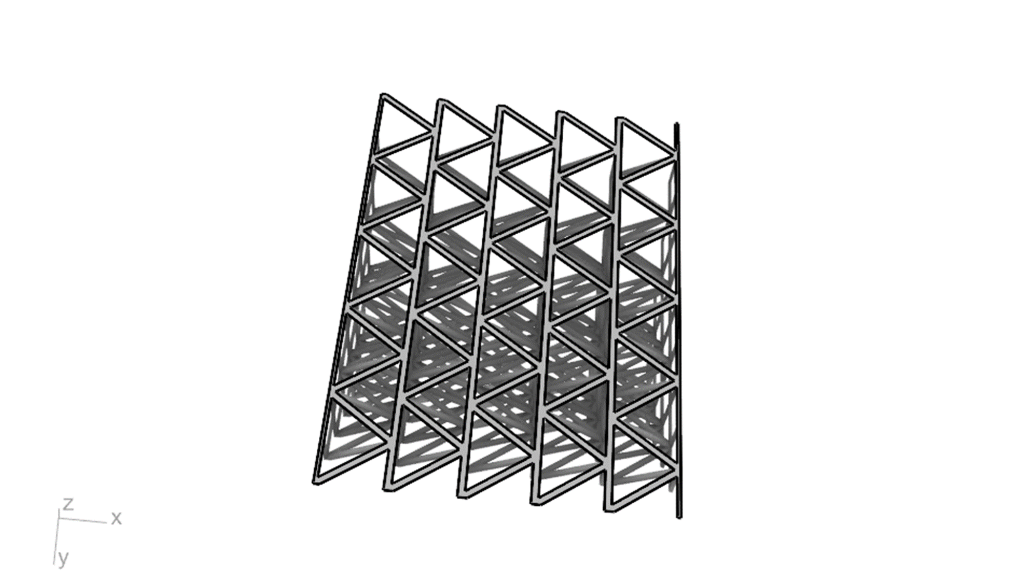
ラティス2
トラスが並んでいる断面(下図3枚目参照、y=z面に平行な面)にがあり、y=z方向近傍で有効的なヤング率が高くなっていると推察できます。


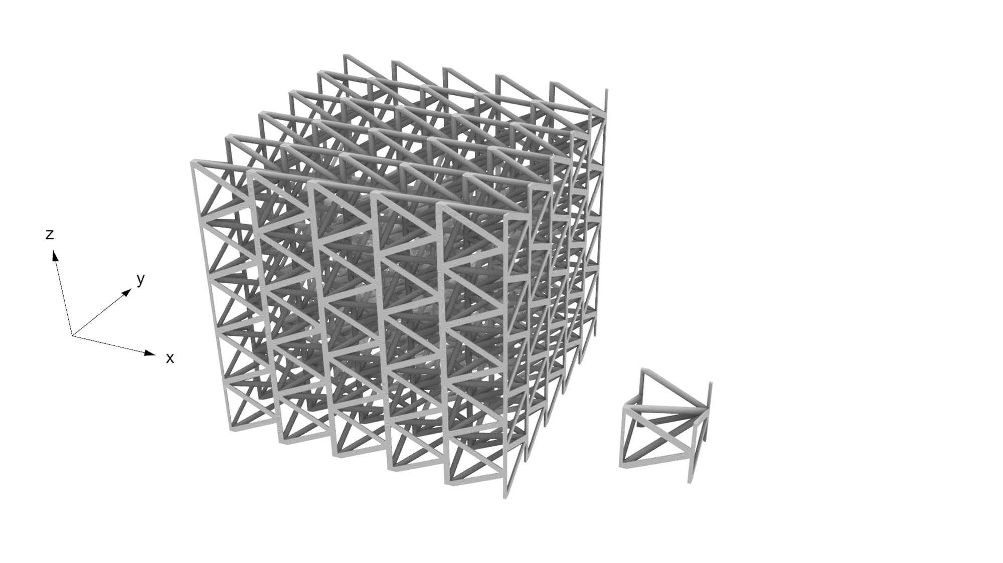
ラティス3
トラスが並んでいる断面(x=0面に平行な面、y=0面に垂直な面)があり、z方向近傍で有効的なヤング率が大きくなっていると推察できます。
最後に
本記事ではラティス構造の弾性行列による均質化と、弾性行列の可視化方法について紹介しました。
均質化を用いると複雑なラティス構造の解析を比較的低い計算コストでできるようになります。
ラティス構造の解析をやってみたい人はぜひ使ってみてください。
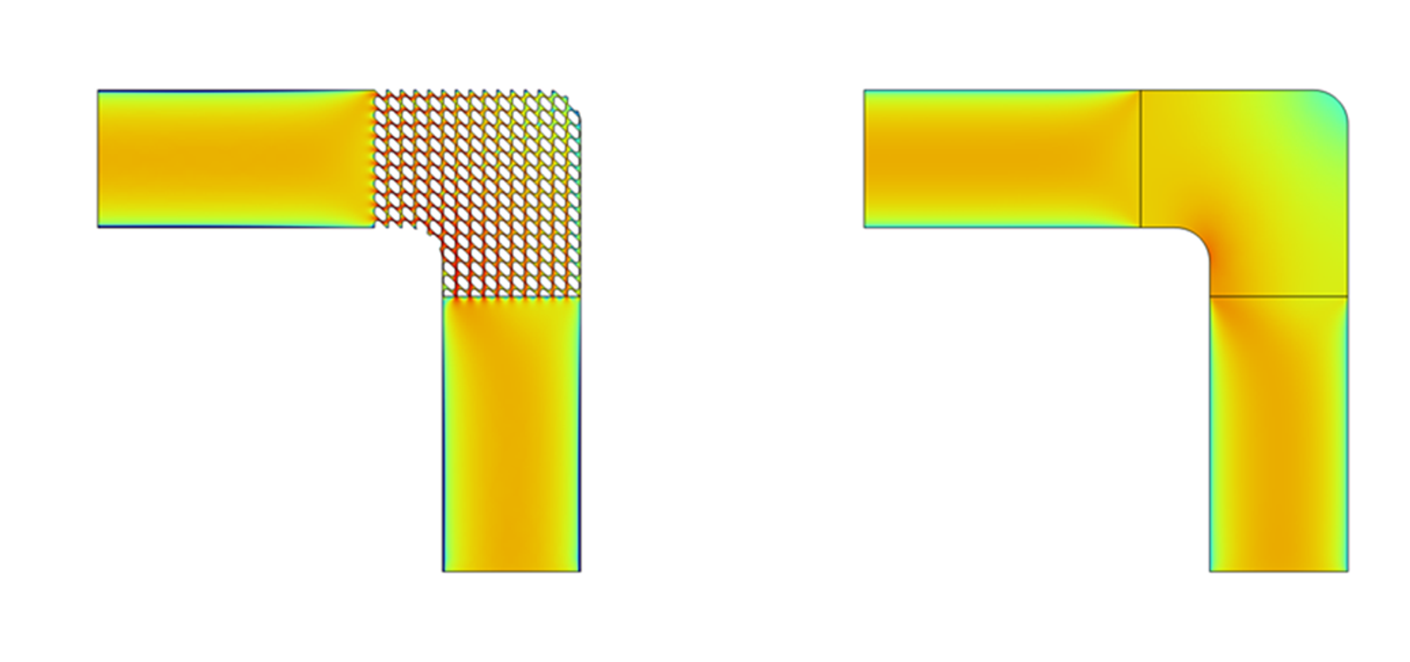
後編では、多孔質モデルによる流路の均質化について紹介します。
Introduction
The topic of homogenization has come up several times in this technical blog.
Homogenizing Mechanical Metamaterial
This article introduces the method of homogenization of lattice structures by numerical experiments and visualization of the results in terms of elastic bodies and fluids (channels).
This article is the first part and introduces homogenization of elastic bodies.
The second part is here: (2) Homogenization of Lattice Structures
Note that while this article introduces homogenization of lattices as an Additive Manufacturing prerequisite,
In client work, it is common to utilize metamaterial structural design techniques while assisting in the development of designs that can be mass-produced at the client's manufacturing facility.
Homogenization of lattice structures into elastic matrices by numerical experiments
There is a homogenization technique that incorporates the behavior of the lattice structure during small deformations into the elasticity matrix.
A numerical experimental approach is often used to obtain elastic matrices equivalent to lattice structures.
Here is an example of one of these numerical experiments.
By Hooke's law, the elastic matrix \(C\) is written as a matrix linking the strain \(\epsilon_{ij}\) and the stress \(\epsilon_{k\ell}\).
\(\begin{align*}
        C
        =
       \left(
            \begin{array}{ccc}
                 c_{xxxx} & c_{xxyy} & c_{xxzz} & c_{xxyz} & c_{xxzx} & c_{xxxy}\\
                 c_{yyxx} & c_{yyyy} & c_{yyzz} & c_{yyyz} & c_{yyzx} & c_{yyxy}\\
                 c_{zzxx} & c_{zzyy} & c_{zzzz} & c_{zzyz} & c_{zzzx} & c_{zzxy}\\
                 c_{yzxx} & c_{yzyy} & c_{yzzz} & c_{yzyz} & c_{yzzx} & c_{yzxy}\\
                 c_{zxxx} & c_{zxyy} & c_{zxzz} & c_{zxyz} & c_{zxzx} & c_{zxxy}\\
                 c_{xyxx} & c_{xyyy} & c_{xyzz} & c_{xyyz} & c_{xyzx} & c_{xyxy}
            \end{array}
        \right)
    \end{align*}\)
\(\begin{align*}
        \left(
            \begin{array}{ccc}
                 \sigma_{xx} \\ \sigma_{yy} \\ \sigma_{zz} \\ \sigma_{yz} \\ \sigma_{zx} \\ \sigma_{xy}
            \end{array}
        \right)
        =
       \left(
            \begin{array}{ccc}
                 c_{xxxx} & c_{xxyy} & c_{xxzz} & c_{xxyz} & c_{xxzx} & c_{xxxy}\\
                 c_{yyxx} & c_{yyyy} & c_{yyzz} & c_{yyyz} & c_{yyzx} & c_{yyxy}\\
                 c_{zzxx} & c_{zzyy} & c_{zzzz} & c_{zzyz} & c_{zzzx} & c_{zzxy}\\
                 c_{yzxx} & c_{yzyy} & c_{yzzz} & c_{yzyz} & c_{yzzx} & c_{yzxy}\\
                 c_{zxxx} & c_{zxyy} & c_{zxzz} & c_{zxyz} & c_{zxzx} & c_{zxxy}\\
                 c_{xyxx} & c_{xyyy} & c_{xyzz} & c_{xyyz} & c_{xyzx} & c_{xyxy}
            \end{array}
        \right)
       \left(
            \begin{array}{ccc}
                 \epsilon_{xx} \\ \epsilon_{yy} \\ \epsilon_{zz} \\ 2\epsilon_{yz} \\ 2\epsilon_{zx} \\ 2\epsilon_{xy}
            \end{array}
        \right)
    \end{align*}\)
The elasticity matrix \(C\) is originally defined for each material, but the behavior of the lattice structure during elastic deformation is included in the \(C\) matrix based on the idea that the lattice structure itself can be considered a homogeneous material when viewed on a macro scale sufficiently larger than the unit size of the lattice structure.
To obtain the elasticity matrix \(C\) homogenizing the Lattice structure, we take the unit structure of the Lattice structure and perform numerical experiments.
After setting the cyclic boundaries of stress and strain at the boundary of the unit structure, the analysis is performed by applying six types of strain as follows.
\(    \begin{align*}
       \left(
            \begin{array}{ccc}
                 \epsilon_{xx} \\ \epsilon_{yy} \\ \epsilon_{zz} \\ 2\epsilon_{yz} \\ 2\epsilon_{zx} \\ 2\epsilon_{xy}
            \end{array}
        \right)
=
       \left(
            \begin{array}{ccc}
                 1 \\ 0\\  0\\ 0 \\ 0 \\ 0
            \end{array}
        \right)
,
       \left(
            \begin{array}{ccc}
                 0 \\ 1\\  0\\ 0 \\ 0 \\ 0
            \end{array}
        \right)
,
       \left(
            \begin{array}{ccc}
                 0 \\ 0\\  1\\ 0 \\ 0 \\ 0
            \end{array}
        \right)
,
       \left(
            \begin{array}{ccc}
                 0 \\ 0\\  0\\ 1 \\ 0 \\ 0
            \end{array}
        \right)
,
       \left(
            \begin{array}{ccc}
                 0 \\ 0\\  0\\ 0 \\ 1 \\ 0
            \end{array}
        \right)
,
       \left(
            \begin{array}{ccc}
                 0 \\ 0\\  0\\ 0 \\ 0 \\ 1
            \end{array}
        \right)
    \end{align*}\)
Calculate the average stress \(\bar{\sigma}^{(n)}_{i,j}\) in each direction, including the void space, for the six types of strain analysis.
Based on the calculated mean stress \(\bar{\sigma}^{(n)}_{i,j}\), a temporary elastic matrix is obtained as follows.
\(\begin{align*}
        \left(
            \begin{array}{ccc}
                 \sigma_{xx} \\ \sigma_{yy} \\ \sigma_{zz} \\ \sigma_{yz} \\ \sigma_{zx} \\ \sigma_{xy}
            \end{array}
        \right)
        =
       \left(
            \begin{array}{ccc}
                 \bar{\sigma}^{(1)}_{xx} & \bar{\sigma}^{(2)}_{xx} & \bar{\sigma}^{(3)}_{xx} & \bar{\sigma}^{(4)}_{xx} & \bar{\sigma}^{(5)}_{xx} & \bar{\sigma}^{(6)}_{xx}\\
\bar{\sigma}^{(1)}_{yy} & \bar{\sigma}^{(2)}_{yy} & \bar{\sigma}^{(3)}_{yy} & \bar{\sigma}^{(4)}_{yy} & \bar{\sigma}^{(5)}_{yy} & \bar{\sigma}^{(6)}_{yy}\\
\bar{\sigma}^{(1)}_{zz} & \bar{\sigma}^{(2)}_{zz} & \bar{\sigma}^{(3)}_{zz} & \bar{\sigma}^{(4)}_{zz} & \bar{\sigma}^{(5)}_{zz} & \bar{\sigma}^{(6)}_{zz}\\
\bar{\sigma}^{(1)}_{yz} & \bar{\sigma}^{(2)}_{yz} & \bar{\sigma}^{(3)}_{yz} & \bar{\sigma}^{(4)}_{yz} & \bar{\sigma}^{(5)}_{yz} & \bar{\sigma}^{(6)}_{yz}\\
\bar{\sigma}^{(1)}_{zx} & \bar{\sigma}^{(2)}_{zx} & \bar{\sigma}^{(3)}_{zx} & \bar{\sigma}^{(4)}_{zx} & \bar{\sigma}^{(5)}_{zx} & \bar{\sigma}^{(6)}_{zx}\\
\bar{\sigma}^{(1)}_{xy} & \bar{\sigma}^{(2)}_{xy} & \bar{\sigma}^{(3)}_{xy} & \bar{\sigma}^{(4)}_{xy} & \bar{\sigma}^{(5)}_{xy} & \bar{\sigma}^{(6)}_{xy}\\
            \end{array}
        \right)
       \left(
            \begin{array}{ccc}
                 \epsilon_{xx} \\ \epsilon_{yy} \\ \epsilon_{zz} \\ 2\epsilon_{yz} \\ 2\epsilon_{zx} \\ 2\epsilon_{xy}
            \end{array}
        \right)
    \end{align*}\)
The elasticity matrix must be symmetric. Even if an element should be zero due to the symmetry of the structure, it will not be zero due to numerical error.
The homogenized elasticity matrix is calculated after adding corrections such as taking the average of symmetric elements.
In the lattice consisting of the beams illustrated above, the actual homogenized elastic matrix for a material with Young's modulus \(7×10^{10}\) Pa and Poisson's ratio \(0.33\) is as follows
\(\begin{align*}
       \left(
            \begin{array}{ccc}
                 4.89×10^8 & 4.73×10^8 & 4.73×10^8 & 0 & 0 & 0\\
                 4.73×10^8 & 4.89×10^8 & 4.73×10^8 & 0 & 0 & 0\\
                 4.73×10^8 & 4.73×10^8 & 4.89×10^8 & 0 & 0 & 0\\
                 0 & 0 & 0 & 4.41×10^8 & 0 & 0\\
                 0 & 0 & 0 & 0 & 4.41×10^8 & 0\\
                 0 & 0 & 0 & 0 & 0 & 4.41×10^8\\
            \end{array}
        \right) .
    \end{align*}\)
Using this elastic matrix, the lattice structure portion of a cantilever beam with a \(5×5\) lattice structure was homogenized and analyzed, results are shown below. (The displacement scaling of boundary conditions and visualization is identical for results with and without homogenization.)
It is clear that the macro deformations are well reproduced.
On the other hand, a plot of von Mises stresses shows the following, indicating that microscopic stresses can no longer be simply estimated due to homogenization.
By performing localized analysis in conjunction with homogenization analysis, microscopic stresses can also be estimated to some extent.
It should also be noted that homogenization assumes a situation where the unit structure of the lattice structure is repeated a sufficiently large number of times, so that homogenization will not be valid if the number of repetitions is small.
Use homogenization with a full understanding of its characteristics.
Visualization of elastic matrices
Next we will show you how to visualize the homogenized elastic matrix.
Since it is difficult to visualize all the information in an elasticity matrix, we consider here the visualization of Young's modulus effectively working in each direction.
As shown in the figure below, the effective Young's modulus in each direction is represented by a point in 2-D or 3-D space that is separated from the origin by a distance corresponding to the Young's modulus in each direction.
Connecting those points to form a line or plane visualizes the effective Young's modulus in each direction.
The effective Young's modulus is defined as the inverse of the diagonal components (\(S_{xx},S_{yy},S_{zz}\)) of the compliance matrix \(S\) (the inverse of the elastic matrix \(C\)) for each direction.
For directions other than `\(x,y,z\), the elasticity matrix is calculated by transforming it according to the coordinate transformations.
This value is Young's modulus itself for isotropic materials
Below we present visualizations of elasticity matrices (Young's modulus) in isotropic and orthotropic materials and in several lattice structures.
Isotropic materials
In isotropic materials, Young's modulus is naturally the same in all directions, and when visualized in three dimensions, the material becomes a sphere.
Orthotropic materials
For orthotropic materials (with \(E_x, E_y, E_z=20, 18, 15\rm{GPa}\),\(\nu_{xy}, \nu_{xy}, \nu_{xz}=0.12,0.10,0.14\) and \(G_{xy}, G_{xy}, G_{xz}=9, 8, 6\rm{GPa}\)) shows that the effective Young's modulus is different in each direction.
Lattice 1
It can be inferred that this lattice structure has a direction in which the beams are aligned, and Young's modulus is greater in that direction.
Lattice 2
truss lined cross section (see the third figure below, parallel to the y=z plane), and it can be inferred that the effective Young's modulus is higher in the vicinity of the y=z direction
Lattice 3
We can infer that the effective Young's modulus is larger in the vicinity of the z direction because of the truss lined cross section (parallel to the x=0 plane and perpendicular to the y=0 plane).
Finally
This article introduced the homogenization of lattice structures by elastic matrices and how to visualize elastic matrices.
Homogenization allows the analysis of complex lattice structures at a relatively low computational cost.
If you are interested in doing an analysis of lattice structures, please use it.
The second part of the presentation will focus on homogenization of channels using a porous model.
