
概要
本技術ブログで、均質化の話題が何度か出ておりました。
(2)アディダス3DPシューズ解説:圧縮力をせん断変形に変換するメカニカルメタマテリアルの設計
本記事では弾性体と流体(流路)の観点で、数値実験によるラティス構造の均質化方法と結果の可視化について紹介します。
本記事は後編で、流体(流路)の均質化について紹介します。
前編はこちら:(1)ラティス構造の均質化
なお、本記事ではAdditive Manufacturing前提となるようなラティスの均質化を紹介しておりますが、
クライアントワークにおいては、メタマテリアル構造設計技術を活用しつつ顧客の製造設備で量産可能な設計開発の支援を行うことが一般的です。
数値実験による流路の均質化
流路の均質化手法として多孔質モデルが一般的に知られています。
多孔質モデルを用いて周期的な流路を均質化する過程を紹介します。
定式化
多孔質体内部の流れにおける流速\(\boldsymbol{v}\)はダルシーの法則(Darcy's law)により表現され、低レイノルズ数において圧力勾配に比例し粘性係数\(\mu\)に反比例することが知られています。
\(\begin{align*}
    {\boldsymbol{v}}=-\frac{\kappa}{\mu}\boldsymbol{\nabla}p
\end{align*}\)
また、ダルシーの法則に慣性の寄与を加えて、圧力損失を速度に比例する粘性項と速度の二乗に比例する慣性項の和で表現したDarcy-Forchheimer equationもあります。
\(\begin{align*}
    \nabla p=-\frac{\mu}{\kappa}v-\frac{\rho}{\kappa'}v^2
\end{align*}\)
多孔質モデルではこれら速度と圧力勾配の関係式をそのまま支配方程式としたり、ナビエ-ストークス方程式の圧力ソース項に入れたりします。
今回は周期的な流路の圧力損失(圧力勾配)を、以下のようにナビエストークス方程式の圧力ソースに入れて定式化します。
\(\begin{align*}
    (\boldsymbol{v}\cdot\nabla) \boldsymbol{v}
    =-\boldsymbol{\nabla} p - \mu\Delta \boldsymbol{v} - \mathbf{\alpha}\boldsymbol{v} - \beta|\boldsymbol{v}|\boldsymbol{v}
\end{align*}\)
\(\alpha\)と\(\beta\)はは多孔質モデルの行列パラメータで、簡単のため定常非圧縮の流れを考えています。
数値実験による多孔質モデルのフィッティング
2次元のラティスを例に均質化過程を紹介します。
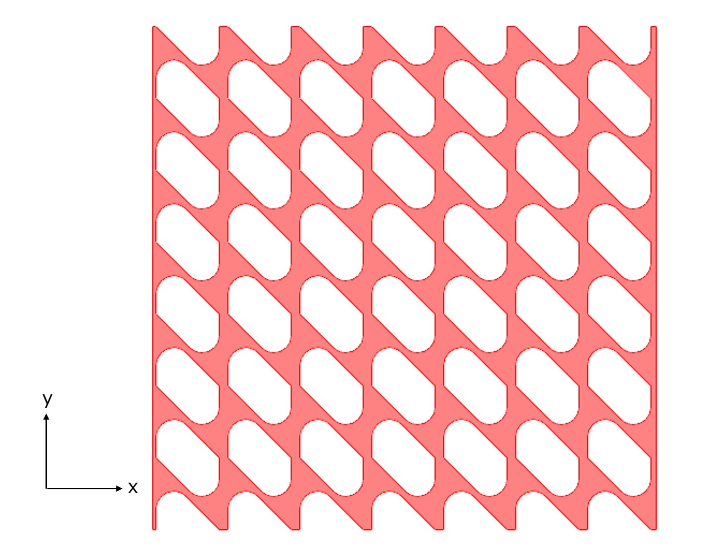
単位構造を取り出すと以下のようになります。

この単位構造の境界速度の周期境界を設定したうえで、下図のように各方向に圧力勾配を加え解析します。
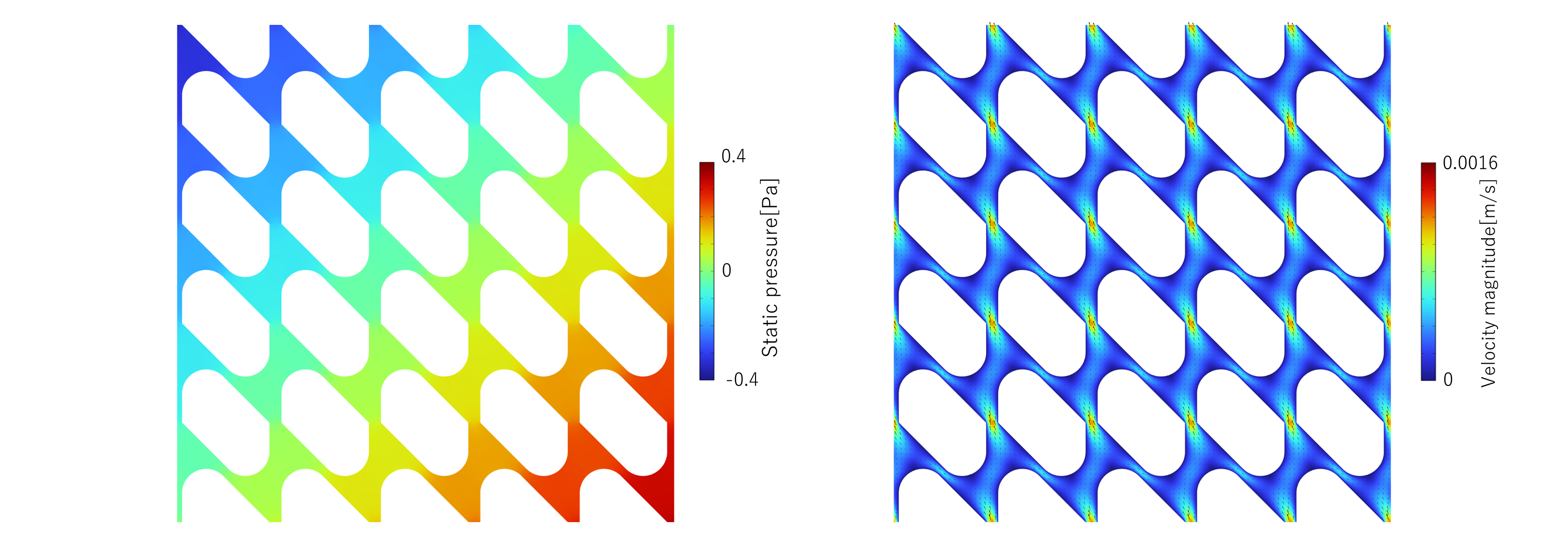
解析した結果をいくつか図示します。
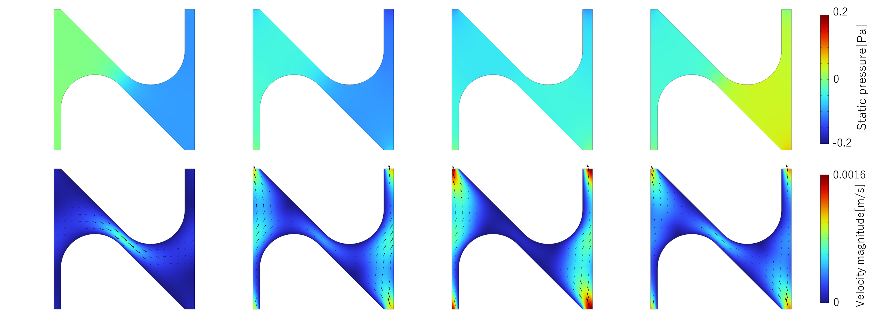
このように各方向の圧力勾配に対して速度場が得られます。
ここでは単位構造の解析をし結果を可視化しましたが、周期境界条件用いているため流路が周期的に繰り返した状況での解析となっています。
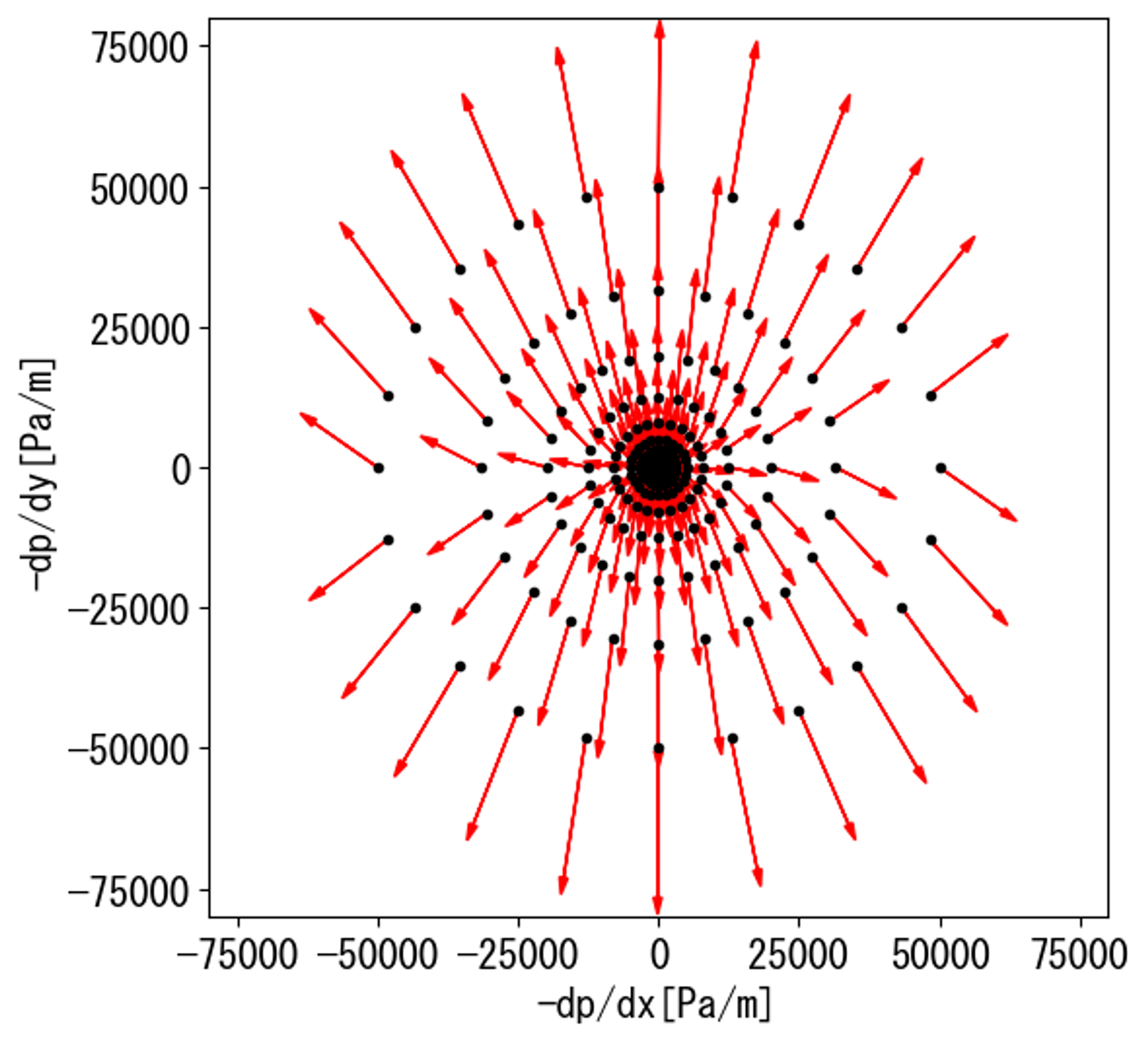
各圧力勾配の解析結果において、非流路部分も含めて速度の平均をとり見かけ速度を見積もります。
入力した圧力勾配とともに、解析結果から得られた見かけ速度を赤矢印の向きと大きさでマッピングすると以下のようになります。
この数値解析で得られた圧力勾配と見かけ速度の結果から、多孔質モデルの行列パラメータ\(\alpha\)と\(\beta\)を算出します。
定式化においてナビエストークス方程式の圧力ソース項に周期流路による圧力損失を入れ込むと説明しましたが、均質化した周期流路による圧力ソースはナビエストークス方程式における粘性項および慣性項より十分大きくなるという考えのもと、均質化のうえではDarcy-Forchheimer equation相当の式でフィッティングをします。
\(\begin{align*}
    \boldsymbol{\nabla} p = - \mathbf{\alpha}\boldsymbol{v} - \beta|\boldsymbol{v}|\boldsymbol{v}
\end{align*}\)
まずは圧力勾配の大きさが500Pa/m以下のデータのみを使用してフィッティングしてみます。
解析結果をもとに見かけの速度を入力、圧力損失を予測する値として線形回帰で\(\alpha\)と\(\beta\)を算出したうえで、"解析の入力圧力損失"と"速度から推定される圧力損失"および"入力圧力損失と推定圧力損失の誤差"をプロットすると以下のようになります。
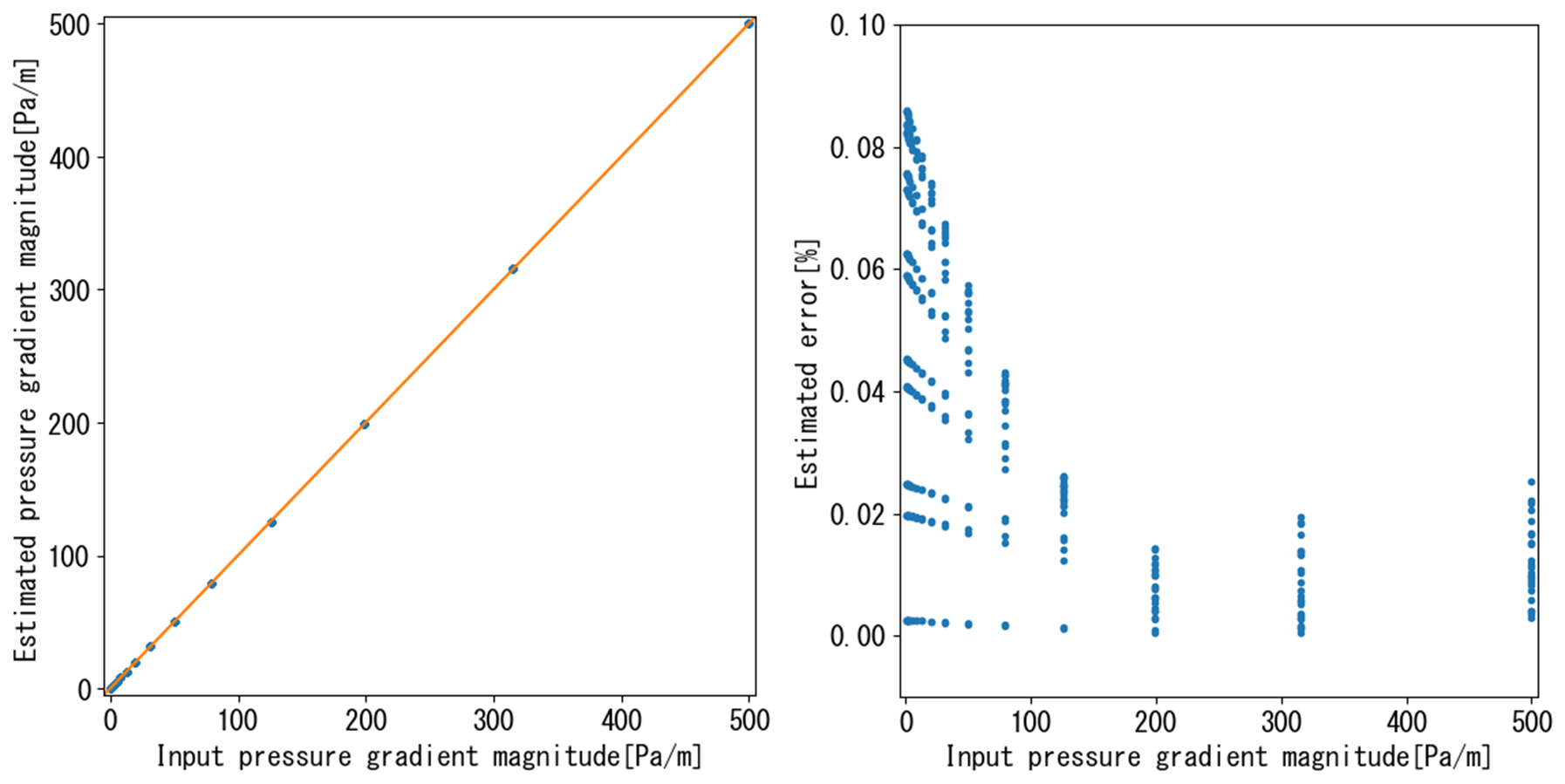
圧力損失が小さく速度が遅い(レイノルズ数が小さい)ときは、ある程度精度よく多孔質モデルにより流れをフィッティングすることができました。
次に、すべてのデータを使用してフィッティングしてみます。
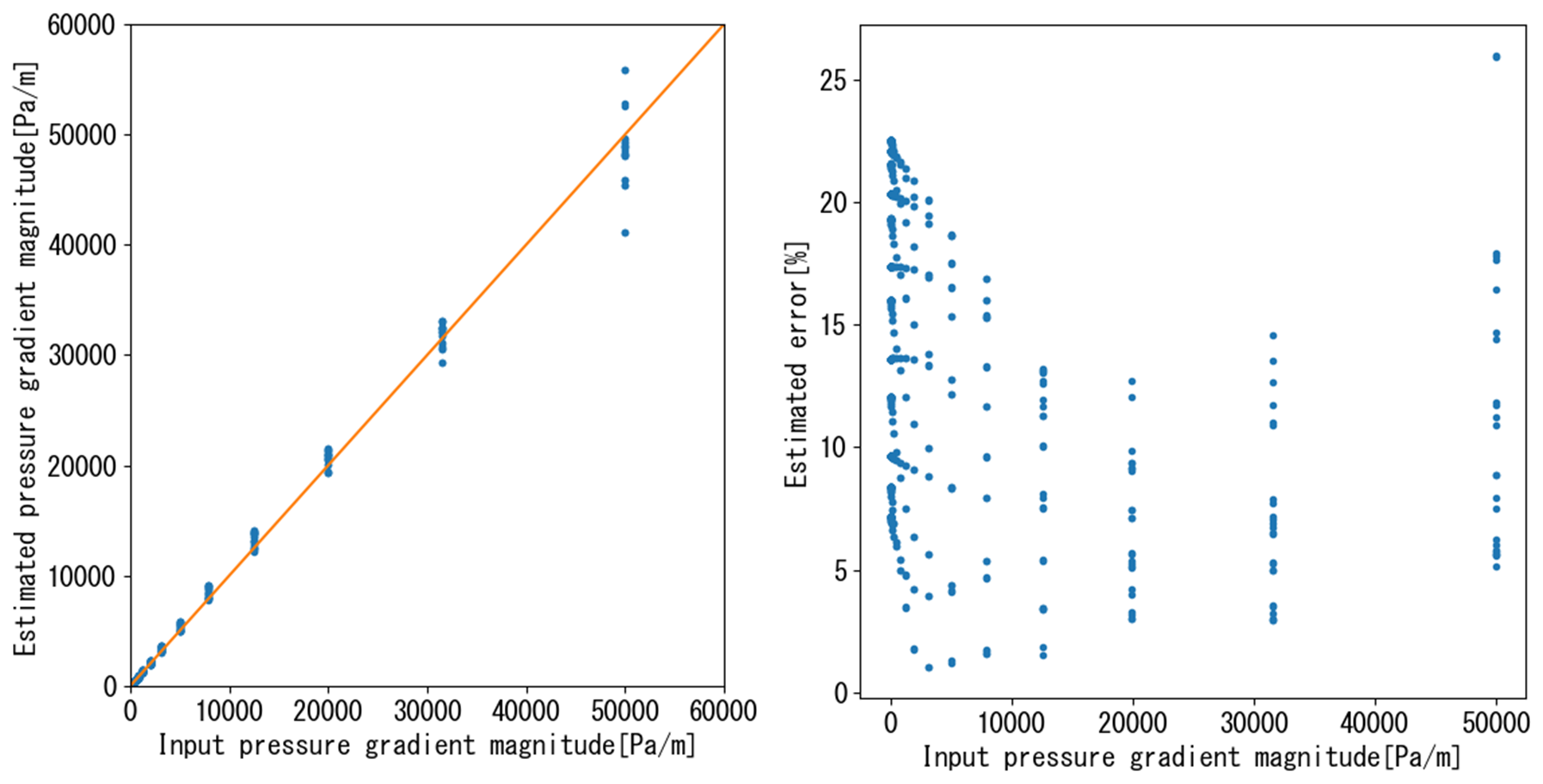
最大で30%近く誤差が出ており、あまり精度よくフィッティングができていません。
圧力勾配が大きいと速度およびレイノルズ数が大きくなり相対的に慣性の寄与が大きくなります。
今回均質化しているラティス構造は慣性により大きく流れの形態が変わりえて、慣性の寄与度に異方性があります。
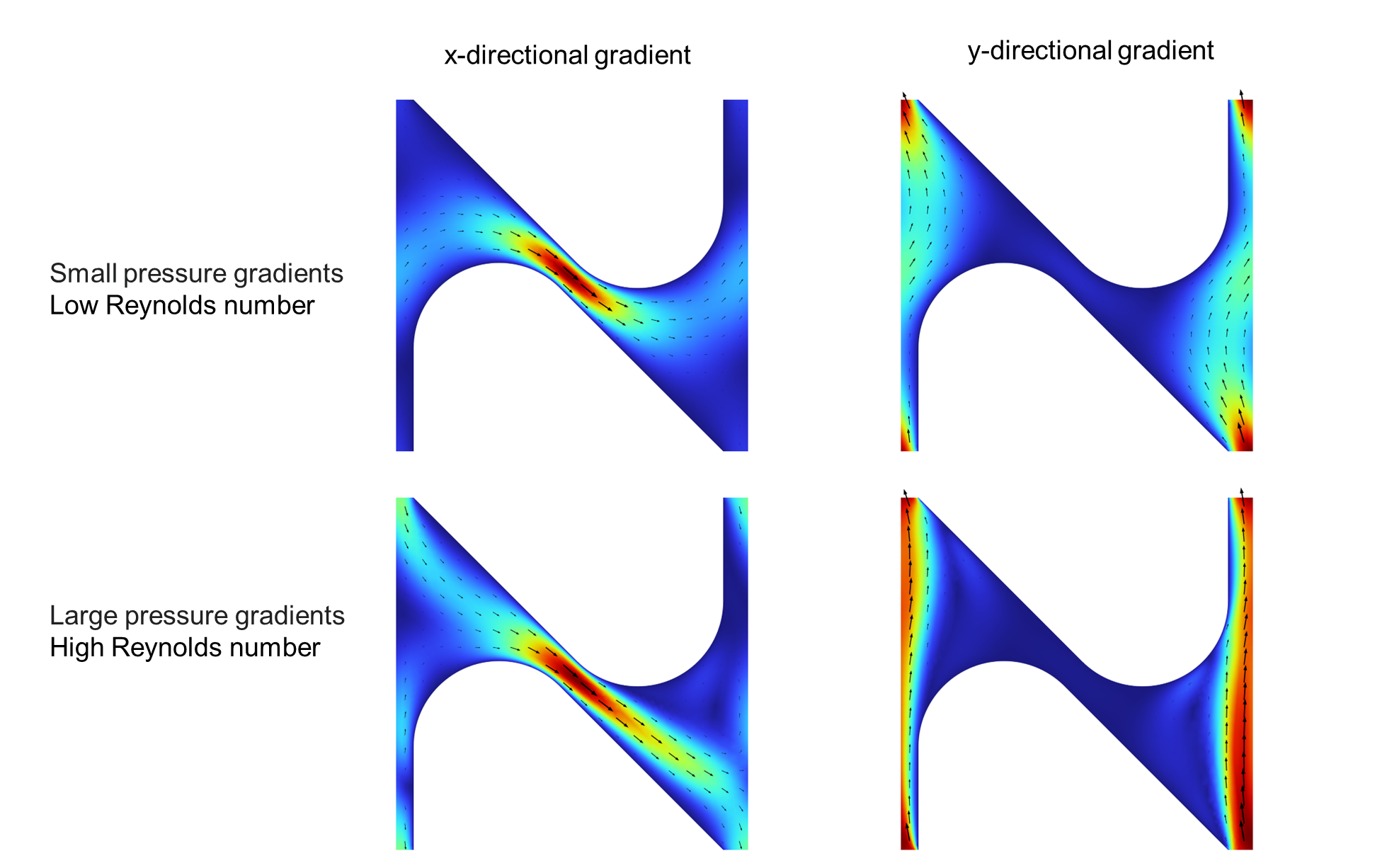
そのため、今回の多孔質モデルの定式化の範囲では流れを表現しきれず誤差が大きくなったと考えられます。
実際に均質化を行う場合は、扱う均質化のモデルが適用できる範囲を注意する必要があります。
多孔質モデルによる解析
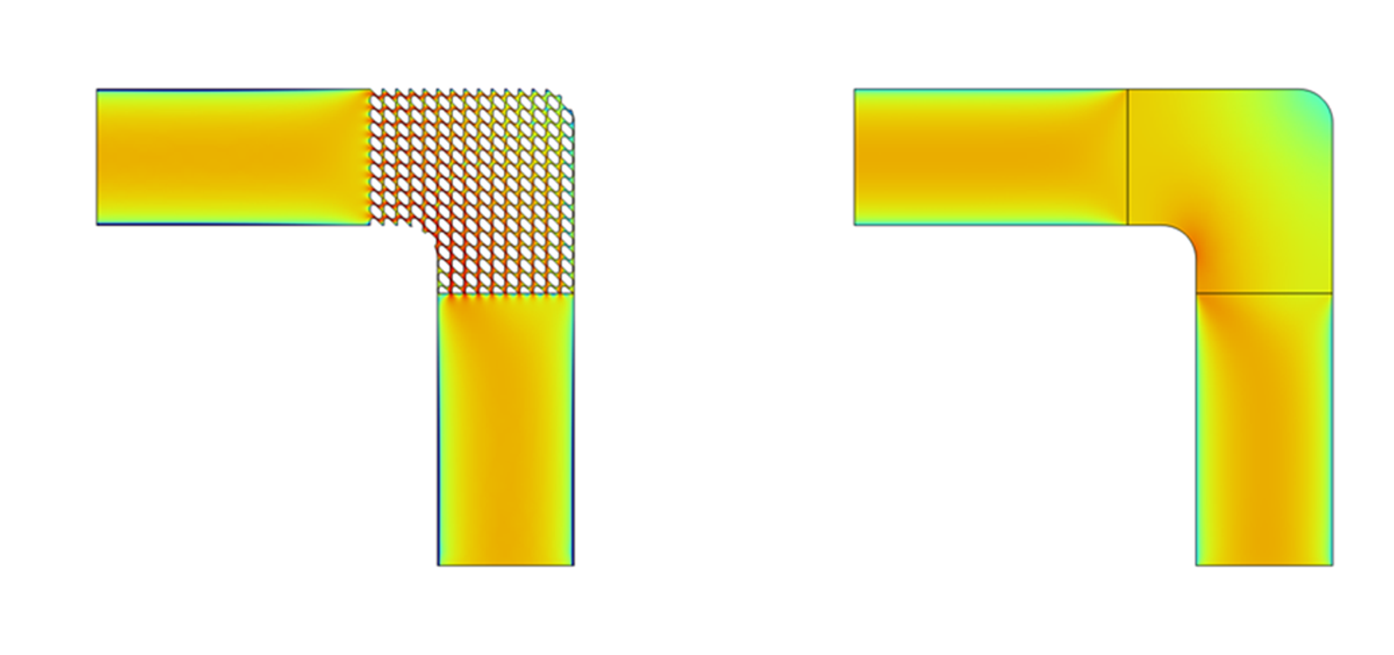
圧力損失500Pa/m以下のデータ使ってフィッティングした多孔質モデルにより、以下の3つの流路の解析を行います。
1,2番目の流路はラティス構造の向きが異なっています。
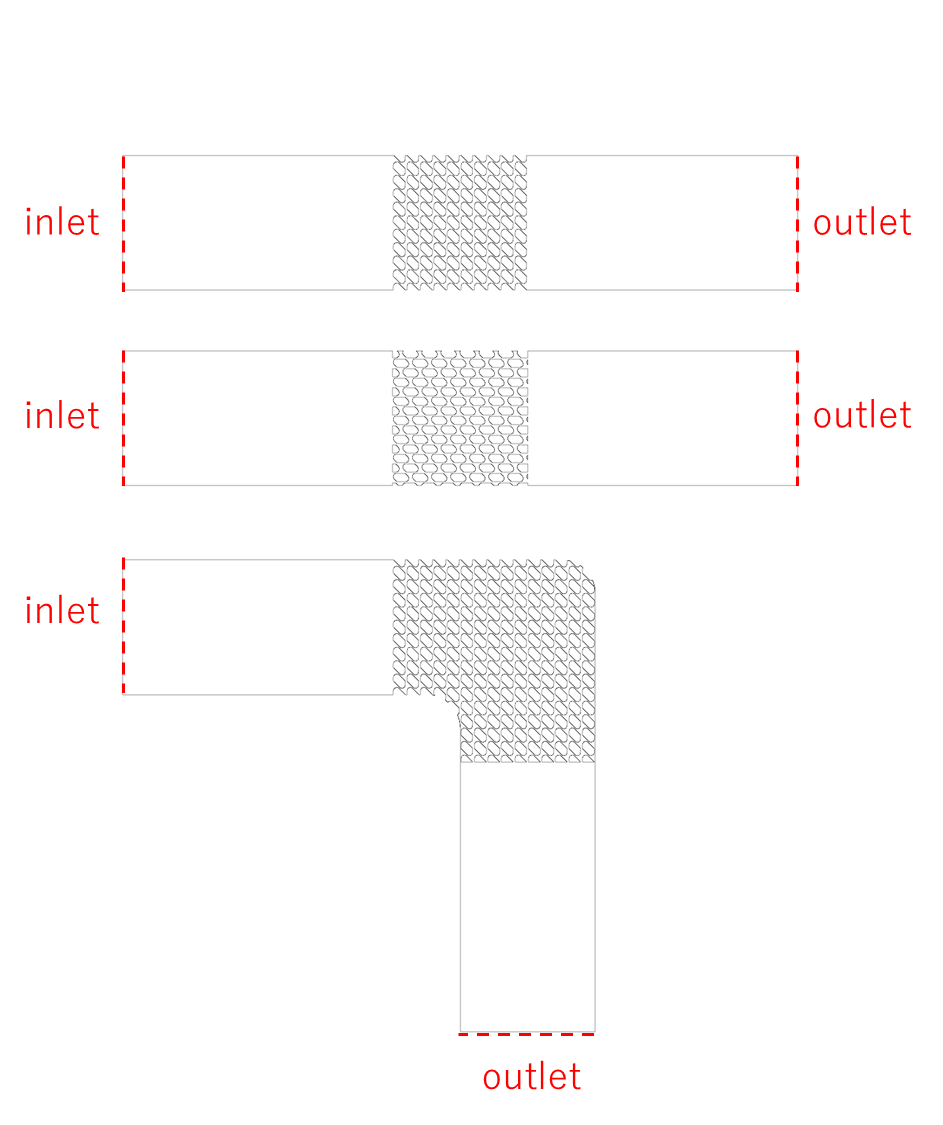
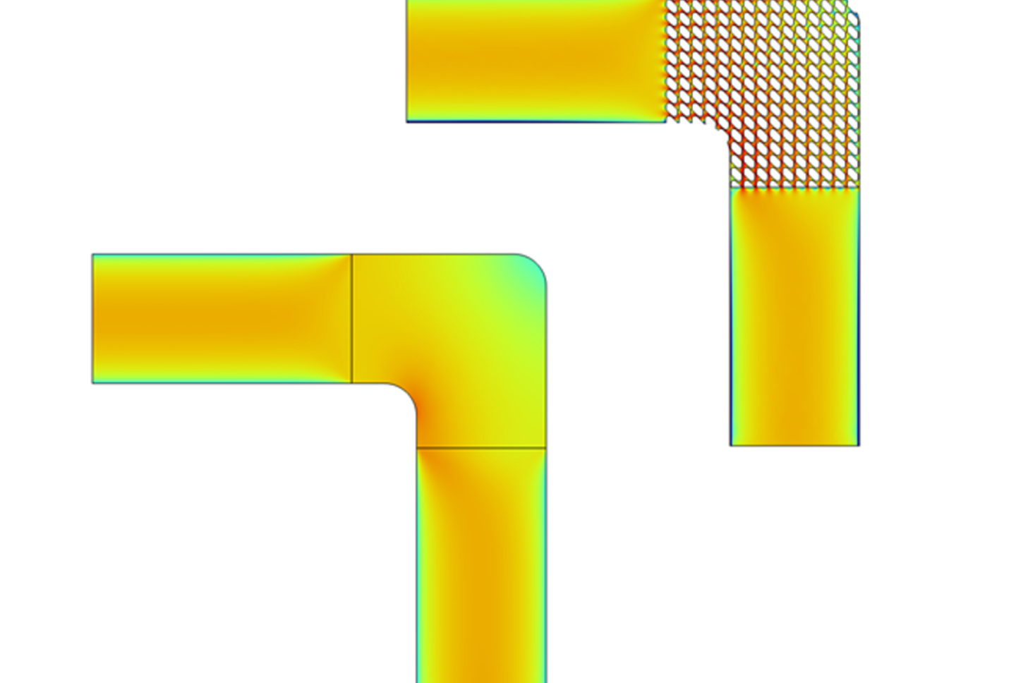
流入口と流出口の圧力差を一定にして解析して、均質化していないものとしたものを比較した結果が以下になります。
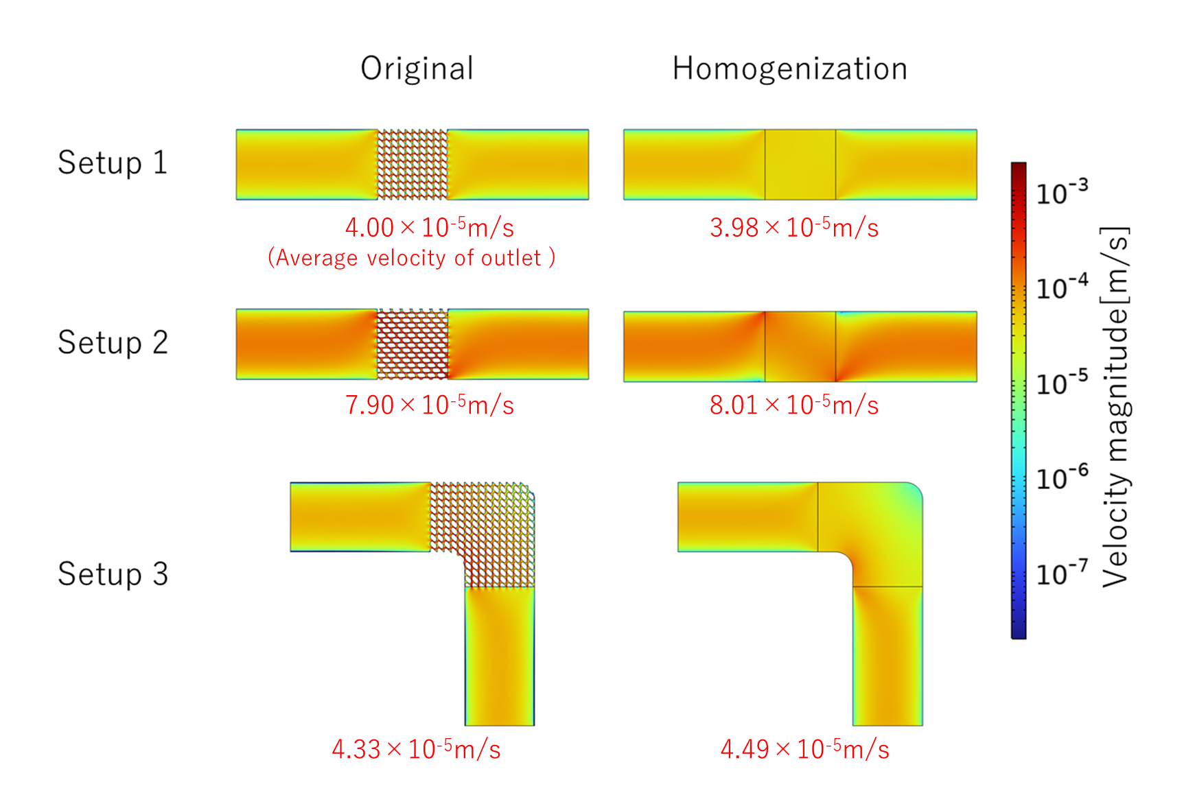
単位構造の繰り返し回数が少ないこともあり多少の差はありますが、多孔質モデルで流れを再現できていることがわかります。
ラティス構造の各方向の流れやすさ可視化
本記事の前編で均質化した弾性行列の可視化を行いました。
同様の可視化手法を用いて、十分流れが遅い状況におけるラティス構造の各方向の流れやすさの可視化を行ってみます。
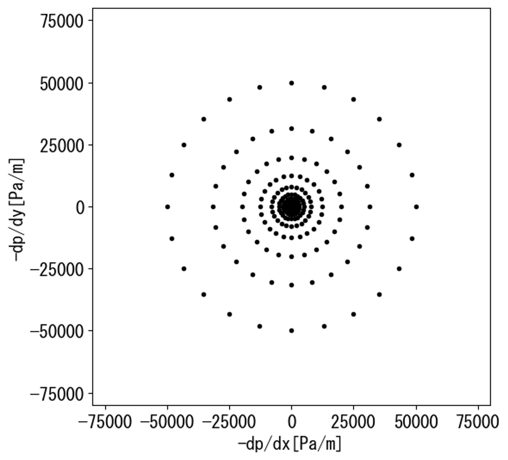
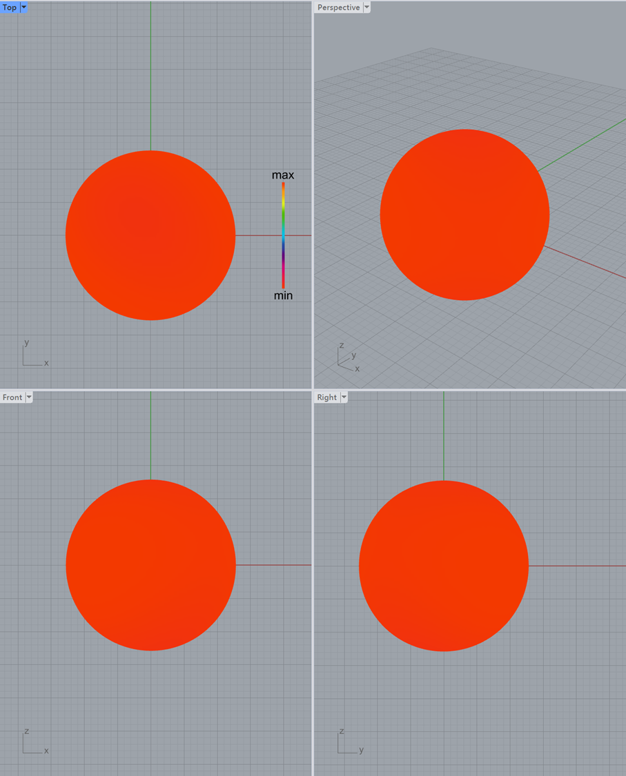
下図のように、各流れの方向に2次元または3次元の空間上で原点からそれぞれの方向に圧力損失に対応する距離だけ離れた点で表現します。
それらの点を結んで線または面にすることで、各方向の流れやすさを可視化します。
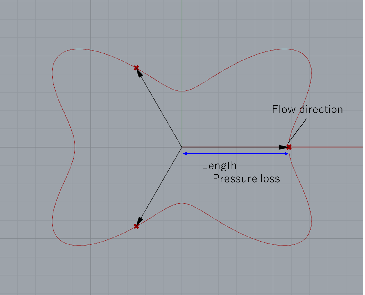
以下でいくつかのラティスについて各方向の流れやすさを可視化します。
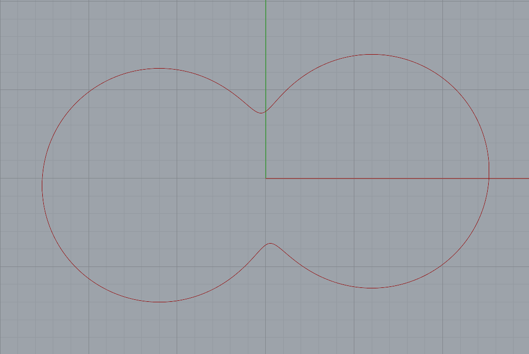
2次元ラティス
上記で均質化した2次元ラティスを均質化します。
3次元ラティス1
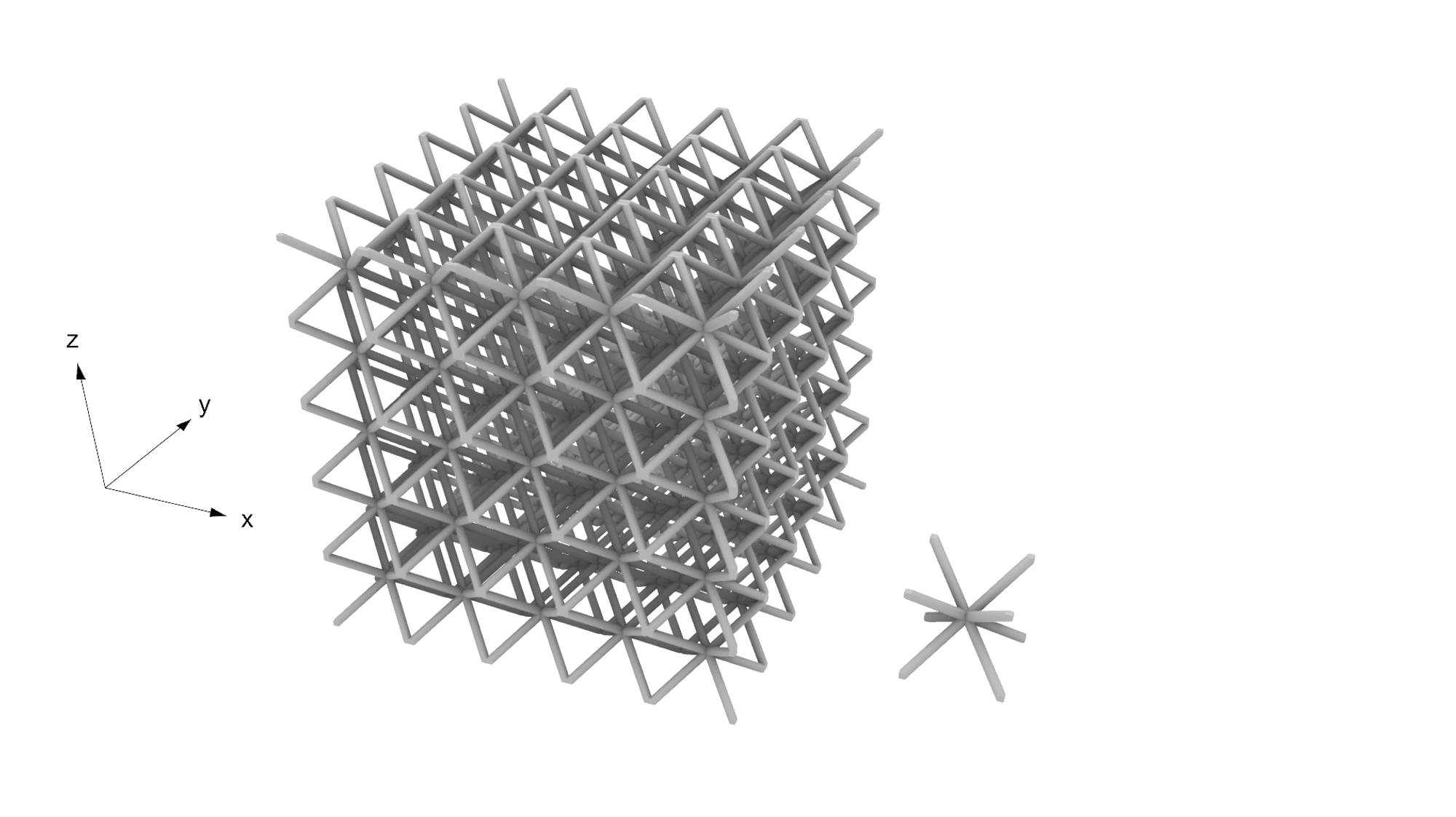
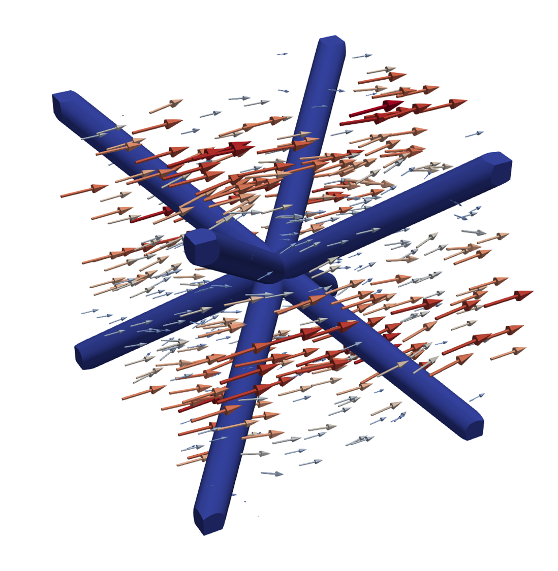
下図1枚目は流路の壁面を、2枚目は解析結果の一例を、3枚目は各方向の流れやすさのを図示しています。
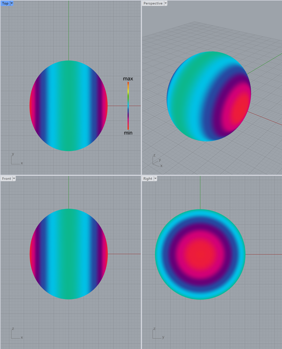
3次元ラティス2
3次元ラティス1と同様に、流路の壁面と各方向の流れやすさを図示しています。

3次元ラティス3
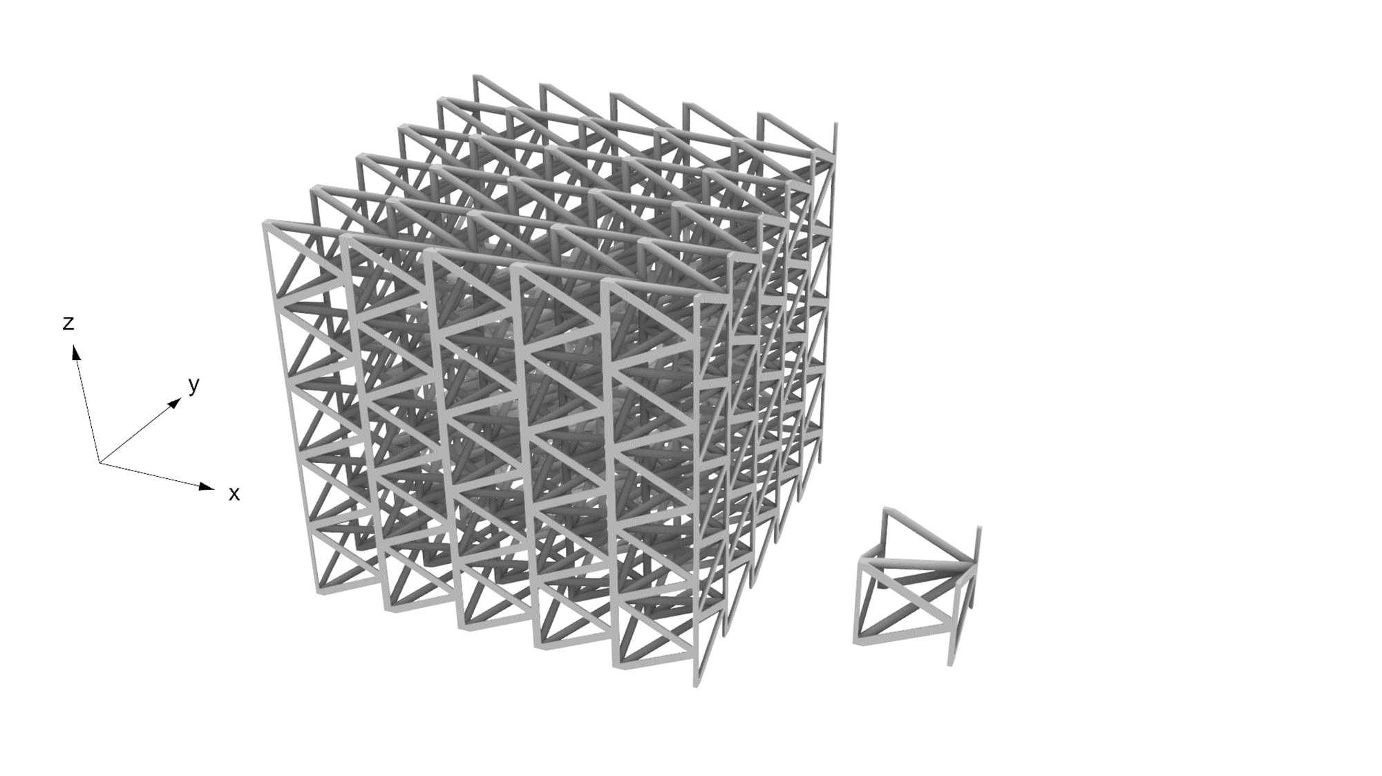
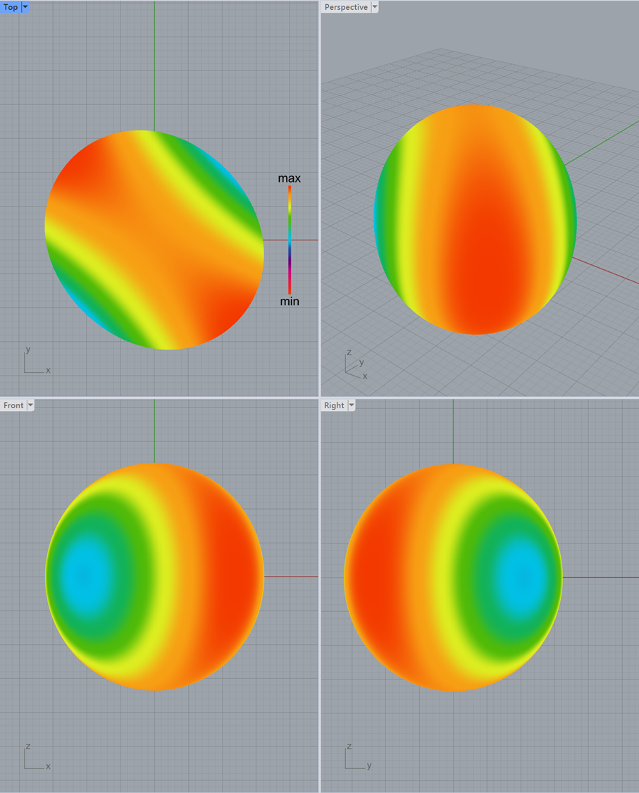
3次元ラティス1,2と同様に、流路の壁面と各方向の流れやすさを図示しています。
最後に
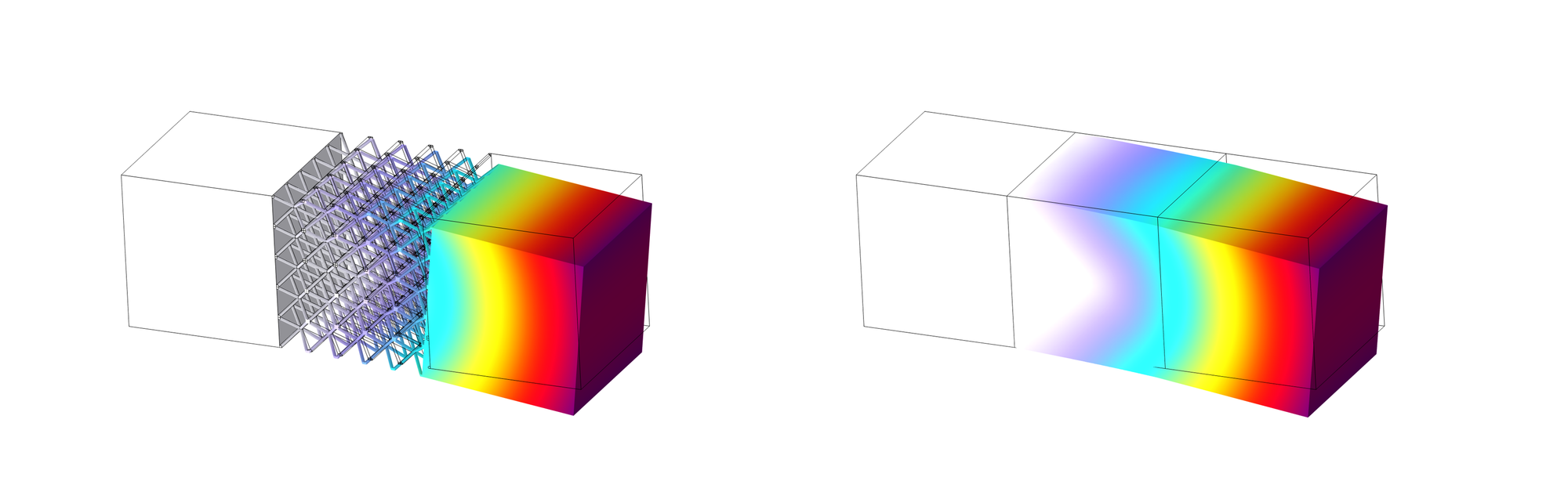
本記事は、前編で構造の弾性行列による均質化と弾性行列の可視化方法について、流路の多孔質モデルによる均質化と各方向の流れやすさの可視化について紹介しました。
均質化は様々な分野で使われ、計算コストを下げるだけでなく、現象の理解にも役立ちます。
興味を持った方はぜひ均質化をやってみて下さい!
Introduction
The topic of homogenization has come up several times in this technical blog.
Homogenizing Mechanical Metamaterial
This article introduces the method of homogenization of lattice structures by numerical experiments and visualization of the results in terms of elastic bodies and fluids (channel).
This article is the second part and introduces homogenization of channels
The first part is here:(1) Homogenization of Lattice Structures
Note that while this article introduces homogenization of lattices as an Additive Manufacturing prerequisite,
In client work, it is common to utilize metamaterial structural design techniques while assisting in the development of designs that can be mass-produced at the client's manufacturing facility.
Homogenization of channels by numerical experiments
The porous model is commonly known as a homogenization method for channels.
This presentation will introduce the process of homogenizing periodic channels using the porous model.
It is known that the flow velocity \(\boldsymbol{v}\) in the porous media is expressed by Darcy's law and is proportional to the pressure gradient and inversely proportional to the viscosity coefficient \(\mu\) at low Reynolds numbers.
\(\begin{align*}
    {\boldsymbol{v}}=-\frac{\kappa}{\mu}\boldsymbol{\nabla}p
\end{align*}\)
There is also the Darcy-Forchheimer equation, which adds an inertial contribution to Darcy's law and expresses the pressure drop as the sum of a viscous term proportional to the velocity and an inertial term proportional to the square of the velocity.
\(\begin{align*}
    \nabla p=-\frac{\mu}{\kappa}v-\frac{\rho}{\kappa'}v^2
\end{align*}\)
relating velocity and pressure gradient can be taken as governing equations as they are, or they can be put into the pressure source term of the Navier-Stokes equation.
In this case, the pressure drop (pressure gradient) in a periodic flow is formulated by putting it into the pressure source of the Navier-Stokes equation as follows.
\(\begin{align*}
    (\boldsymbol{v}\cdot\nabla) \boldsymbol{v}
    =-\boldsymbol{\nabla} p - \mu\Delta \boldsymbol{v} - \mathbf{\alpha}\boldsymbol{v} - \beta|\boldsymbol{v}|\boldsymbol{v}
\end{align*}\)
\(\alpha\) and \(beta\) are the matrix parameters of the porous model, and for simplicity we consider a steady uncompressed flow.
Numerical Experiments Fitting Porous Models
The homogenization process is presented using a 2-dimensional lattice as an example.
The unit structure can be taken out as follows
After setting the periodic boundary of the boundary velocity of this unit structure, a pressure gradient is added in each direction for analysis as shown in the figure below.
Some of the results of the analysis are illustrated in the following figures.
Thus, velocity fields are obtained for pressure gradients in each direction.
Here, the unit structure is analyzed and the results are visualized, but because periodic boundary conditions are used, the analysis is based on a situation in which the flow path repeats itself periodically.
In the analysis results for each pressure gradient, the apparent velocity is estimated by averaging the velocities, including the non-flow path portion.
The apparent velocity obtained from the analysis results, along with the input pressure gradient, is mapped with the direction and magnitude of the red arrow as shown below.
From the pressure gradient and apparent velocity results obtained from this numerical analysis, the matrix parameters \(\alpha\) and \(beta\) of the porous model are calculated.
In the formulation, it is explained that the pressure drop due to the periodic channel is included in the pressure source term of the Navier-Stokes equation, but based on the idea that the pressure source due to the homogenized periodic channel is sufficiently larger than the viscous and inertial terms in the Navier-Stokes equation, the Darcy-Forchheimer equation is used for fitting.
\(\begin{align*}
    \boldsymbol{\nabla} p = - \mathbf{\alpha}\boldsymbol{v} - \beta|\boldsymbol{v}|\boldsymbol{v}
\end{align*}\)
First, try fitting using only data with pressure gradients of 500 Pa/m or less.
The apparent velocity is input based on the analysis results, and \(\alpha\) and \(\beta\) are calculated by linear regression as values to predict the pressure drop. The plot is as follows.
When the pressure drop is small and the velocity is slow (small Reynolds number), the flow could be fitted by the porous model with some accuracy.
Next, let us try fitting using all the data.
The maximum error is nearly 30%, which is not a very accurate fitting.
The larger the pressure gradient, the larger the velocity and Reynolds number, and the larger the relative contribution of inertia.
In the lattice structure homogenized in this study, inertia can significantly change the flow pattern, and the contribution of inertia is anisotropic.
Therefore, it is believed that the range of the formulation of the porous model in this case was not sufficient to represent the flow, resulting in a large error.
When actually performing homogenization, one should be careful about the applicable range of the homogenization model to be handled.
Porous model analysis
The following three channels are analyzed using a porous model fitted with data for pressure drop less than 500 Pa/m.
The first and second channels have different lattice structure orientations.
The following is the result of an analysis with a constant pressure difference between the inlet and outlet and a comparison of the non-homogenized and homogenized results.
Although there are some differences due to the small number of iterations of the unit structure, it is clear that the porous model is able to reproduce the flow.
Visualization of ease of flow in each direction of lattice structure
We visualized the homogenized elastic matrix in the first part of this article.
Using the same visualization technique, we will try to visualize the ease of flow in each direction of the lattice structure in a sufficiently slow flow situation.
As shown in the figure below, each flow direction is represented by a point in 2-D or 3-D space separated from the origin by a distance corresponding to the pressure drop in each direction.
By connecting those points to form a line or a plane, the ease of flow in each direction is visualized.
Below we visualize the ease of flow in each direction for several lattices.
2D Lattice
Homogenize the 2D lattice homogenized above.
3D Lattice 1
The first figure below shows the wall surface of the channel, the second shows an example of the analysis results, and the third illustrates the ease of flow in each direction.
3D Lattice 2
As in 3D Lattice 1, the walls of the channel and the ease of flow in each direction are illustrated.
3D Lattice 3
As in 3D Lattice 1 and 2, the walls of the channel and the ease of flow in each direction are illustrated.
Finally
In the first part of this article, homogenization by elastic matrices of structures and methods of visualizing elastic matrices were introduced, as well as homogenization by porous models of channels and visualization of flow ease in each direction.
Homogenization is used in various fields and helps not only to reduce computational cost but also to understand phenomena.
If you are interested, please try homogenization!
