はじめに

まずは次の動画をご覧ください。

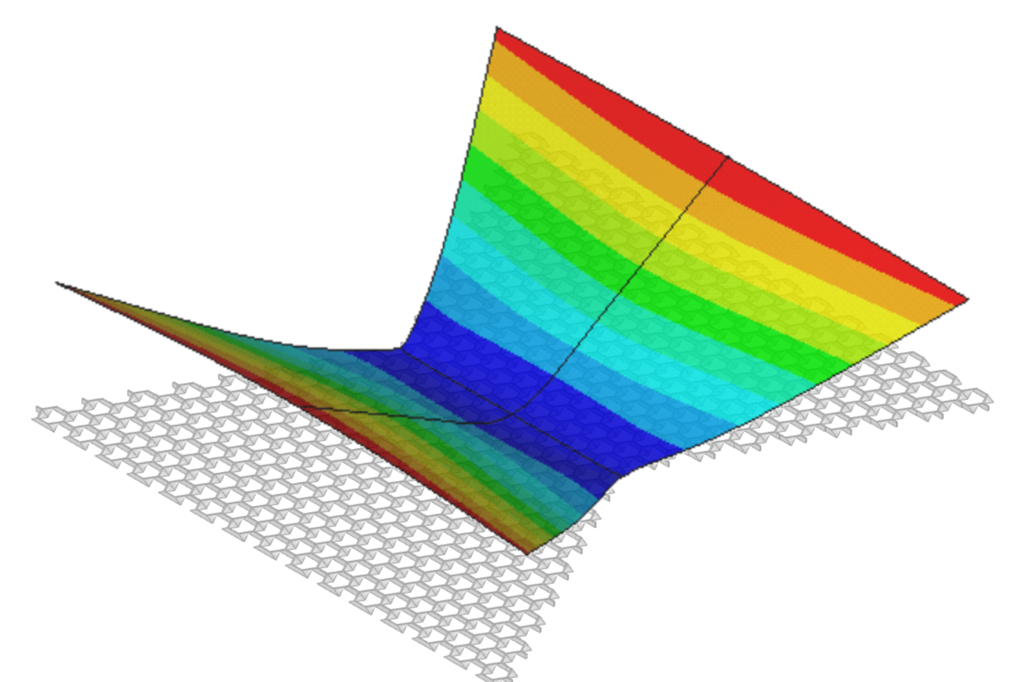
動画で紹介された構造は，面内荷重によって面外変形を起こす機能を持つメタマテリアル（弊社特許取得済み，特許第7229616号）を使用しています。 本記事では，このメタマテリアルの基本構造や簡易解析法を紹介いたします。

参考

• Imperial College London. Shell metamaterials.(参照2023年09月)
• Rob Hewson. Multiscale Actuated Shells Structures. 15th World Congress on Computational Mechanics, 2022

基本構造

ハニカム，リエントラントハニカム

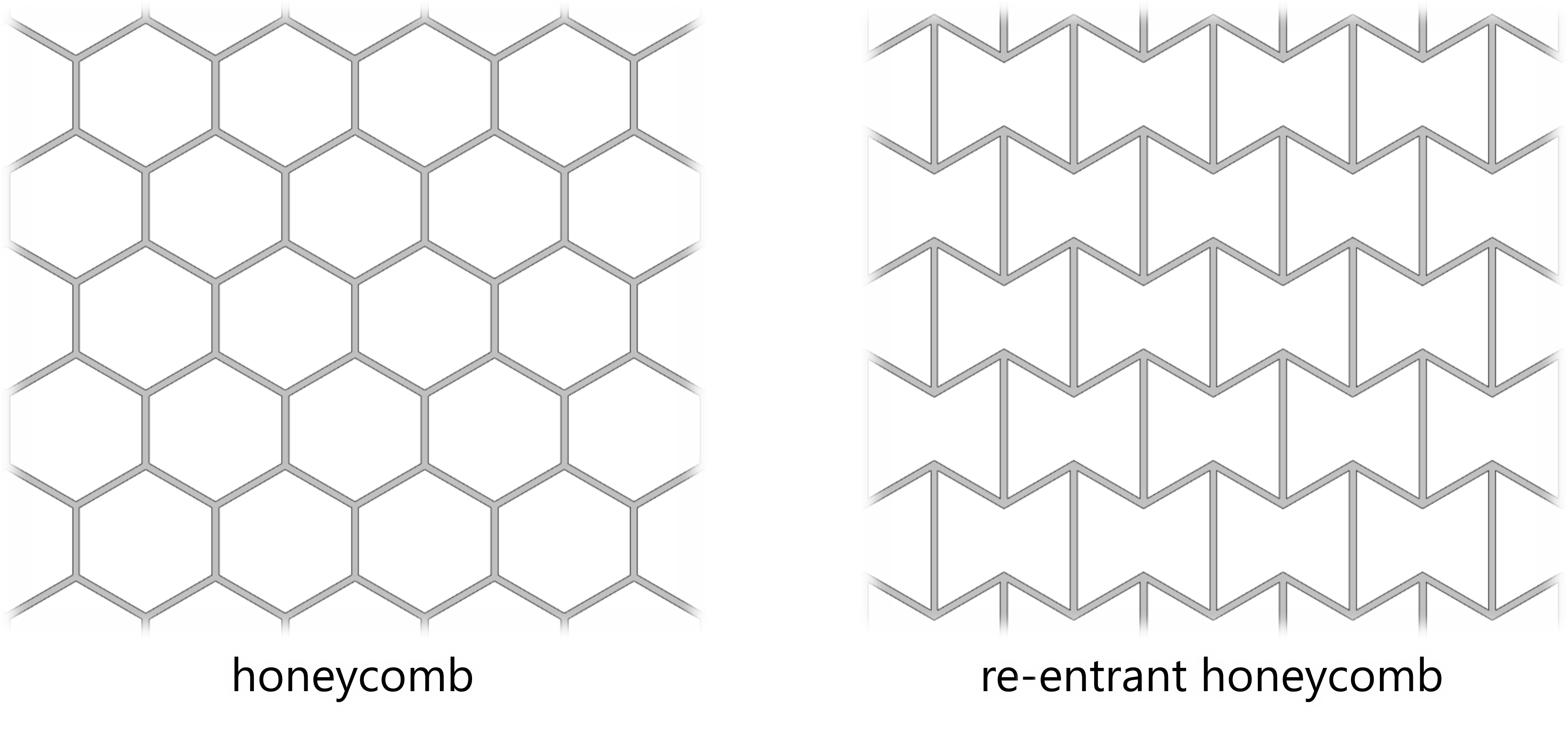
本記事の動画に出てきた構造はすべてハニカムを基本とした形状となっています。ハニカム形状は，六角形のセルが密に詰まった，空間を効率的に利用できるパターンとして広く利用されています。

通常のハニカムはポアソン比は正の値を取りますが，角度を変えるとポアソン比が負になります。これはリエントラントハニカムと呼ばれ，代表的なAuxetic構造（ポアソン比が負の構造）の一つです。

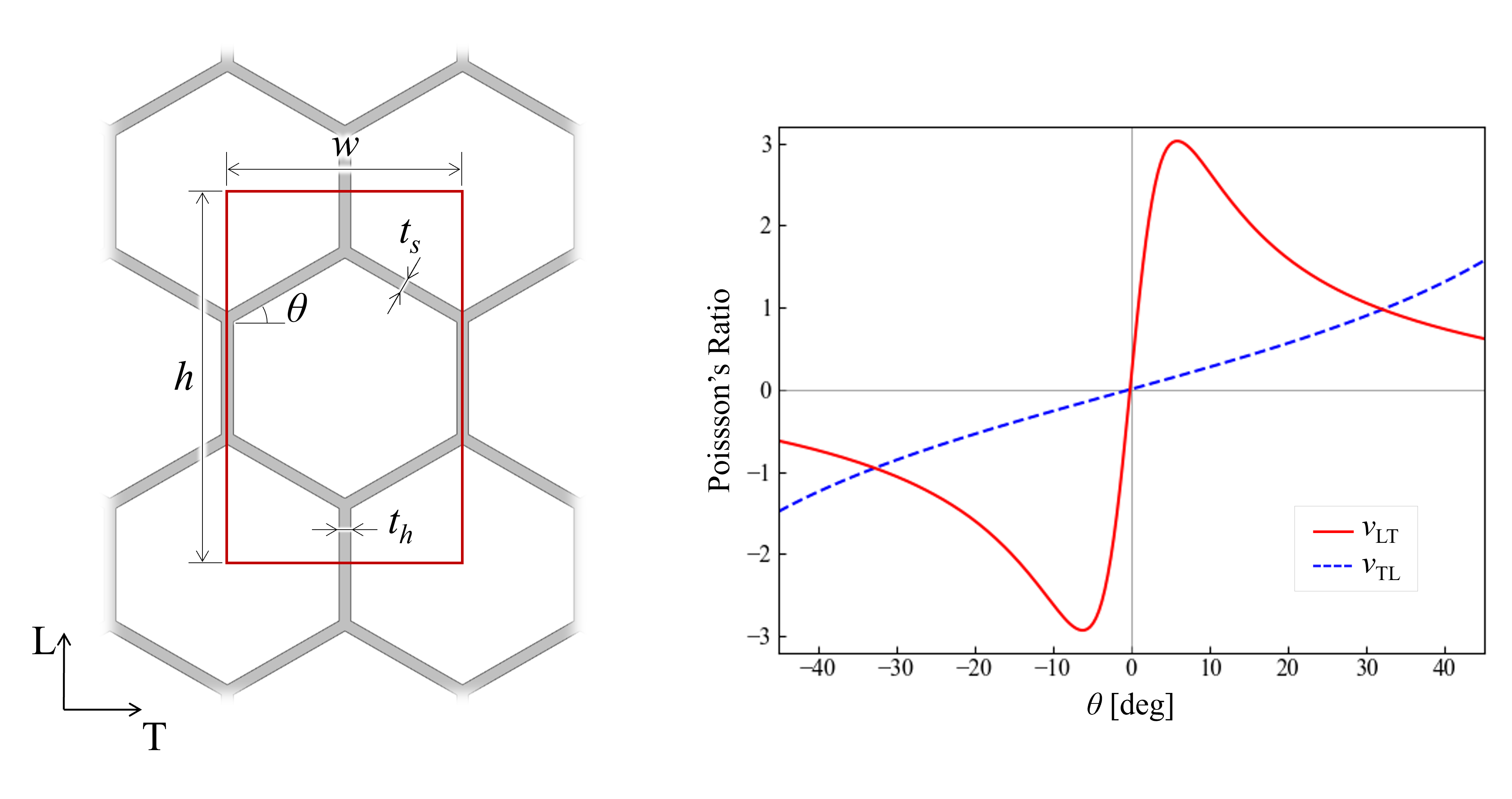
実際に，有限要素解析を用いて角度を変化させたときのポアソン比を求めてみます。下図の赤線で囲った単位構造の大きさを変化させないように斜め梁の中央位置を固定し，角度θを変化させます。h=1.6w, t_h=t_s=0.05wとしたとき，各方向のマクロなポアソン比は下図のようになりました。ν_{LT}, ν_{TL}はそれぞれ，L方向負荷時のT方向ひずみ，T方向負荷時のL方向ひずみを表すポアソン比です。基本的にθが正のときにポアソン比が正，θが負のときにポアソン比が負となることが分かります。

このように，単位構造の寸法を変化させることで，マクロ物性を連続的に変えることができます。

変形メカニズム

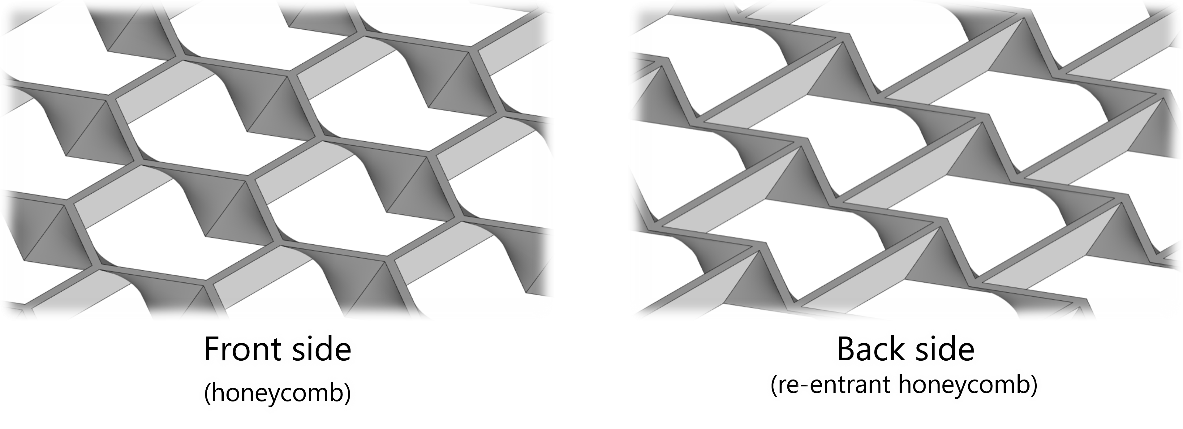
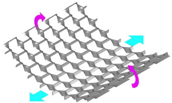
面内荷重によって面外に変形するメタマテリアルの基本構造は，片面をポアソン比が正のハニカム構造，もう一方の面をポアソン比が負のリエントラントハニカム構造となるように形状を滑らかに繋げています。

引張荷重が負荷された際に，ハニカム側の面が直交方向に収縮し，リエントラントハニカム側の面が膨張するため，全体的に曲げ変形が生じる構造となっています。

均質化法

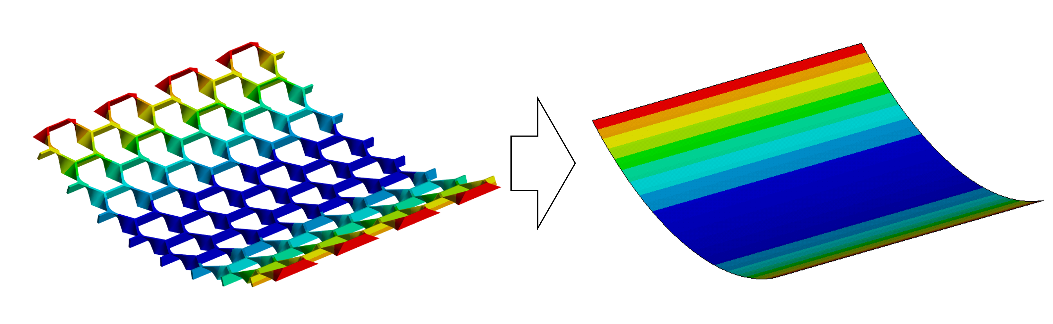
均質化法とは，複雑な微細構造を持つ材料や構造の特性を，よりシンプルな等価的な均質材料の特性に変換する方法です。これにより，材料全体の挙動を理解することが可能となります。また，均質化法を用いることで，複雑な微細構造を持つ材料の解析を簡素化し計算コストを削減することができます。上のグラフで示したポアソン比の算出も，2次元平面内での均質化と言えます。

今回は，薄板のような形状を扱うため，シェル要素を用いてモデルを作成します。弾性変形を仮定した場合，シェル要素の特性は次のように表現できます。

\begin{bmatrix} [N] \\ [M] \end{bmatrix}
=
\begin{bmatrix} 
[A] & [B] \\ [B] & [D]
\end{bmatrix}
\begin{bmatrix} 
[\varepsilon] \\ [\kappa]
\end{bmatrix}
=
\begin{bmatrix} 
a_{11} & a_{12} & a_{16} & b_{11} & b_{12} & b_{16} \\
a_{12} & a_{22} & a_{26} & b_{12} & b_{22} & b_{26} \\
a_{16} & a_{26} & a_{66} & b_{16} & b_{26} & b_{66} \\
b_{11} & b_{12} & b_{16} & d_{11} & d_{12} & d_{16} \\
b_{12} & b_{22} & b_{26} & d_{12} & d_{22} & d_{26} \\
b_{16} & b_{26} & b_{66} & d_{16} & d_{26} & d_{66} \\
\end{bmatrix}
\begin{bmatrix} 
\varepsilon_{x} \\ \varepsilon_{x}\\ \gamma_{xy}\\
\kappa_{x} \\ \kappa_{y} \\ \kappa_{xy}

\end{bmatrix}

ここで，[N]と[M]は単位長さあたりの面内荷重とモーメント，[\varepsilon]と[\kappa]は中立面での面内ひずみと曲率を表します。[A], [B], [D]はそれぞれ面内剛性行列、カップリング行列，曲げ剛性行列と呼ばれます。 また，今回は横せん断変形も考慮します。

\begin{bmatrix} [V]\end{bmatrix}
=
\begin{bmatrix} 
[K]
\end{bmatrix}
\begin{bmatrix} 
[\gamma]
\end{bmatrix}
=
\begin{bmatrix} 
a_{55} & a_{45}\\
a_{45} & a_{44}
\end{bmatrix}
\begin{bmatrix} 
\gamma_{zx}\\ \gamma_{yz}
\end{bmatrix}

[V]は単位長さあたりの横せん断力を、[\gamma]は横せん断ひずみを表します。等方性材料の場合，横せん断剛性行列[K]は横弾性係数Gに板厚tを乗じた値を成分に持つ対角行列となります。

\begin{bmatrix}
[K]
\end{bmatrix}
=
\begin{bmatrix}
Gt & 0\\
0 & Gt
\end{bmatrix}

これらの剛性行列を計算することで，マクロスケールでの挙動を簡易的にシミュレーションすることができます。

古典積層理論

今回は，古典積層理論を用いて剛性マトリクスを算出します。古典積層理論は，複合材料積層板に対してよく用いられ，平面応力状態の板の弾性特性（面内剛性や曲げ剛性）を簡便に導出する手法です。

中立面での面内ひずみ[\varepsilon]と曲率[\kappa]が与えらた場合，中立面からzの位置にある面でのひずみは次のように与えらえます。

\begin{bmatrix}
\varepsilon_{x} \\ \varepsilon_{y} \\ \gamma_{xy}
\end{bmatrix}+
z\begin{bmatrix}
\kappa_{x} \\ \kappa_{y} \\ \kappa_{xy}
\end{bmatrix}

このとき，応力の積分値が外力とつり合うことを考えると，単位長さあたりの面内荷重[N]およびモーメント[M]は，位置zにおける面内剛性行列[Q]を用いて次のように表されます。ただし，以下では中立面と中央面が一致すると仮定します。

N_i = 
\int_{-t/2}^{t/2}\sigma_{i}dz=
\left(\int_{-t/2}^{t/2}Q_{ij}dz\right)\varepsilon_{i}+
\left(\int_{-t/2}^{t/2}Q_{ij}zdz\right)\kappa_{i}\\
M_i = 
\int_{-t/2}^{t/2}\sigma_{i}zdz=
\left(\int_{-t/2}^{t/2}Q_{ij}zdz\right)\varepsilon_{i}+
\left(\int_{-t/2}^{t/2}Q_{ij}z^2dz\right)\kappa_{i}

これをもとに，上述した面内剛性行列[A]，カップリング行列[B]，曲げ剛性行列[D]はそれぞれ次のように導出できます。

A_{ij} = \int_{-t/2}^{t/2}Q_{ij}dz =
\sum_{k=1}^{N}Q_{ij}^{(k)}(z_k-z_{k-1})\\
B_{ij} = \int_{-t/2}^{t/2}Q_{ij}zdz =
\frac{1}{2}\sum_{k=1}^{N}Q_{ij}^{(k)}(z_k^2-z_{k-1}^2)\\
D_{ij} = \int_{-t/2}^{t/2}Q_{ij}z^2dz =
\frac{1}{3}\sum_{k=1}^{N}Q_{ij}^{(k)}(z_k^3-z_{k-1}^3)

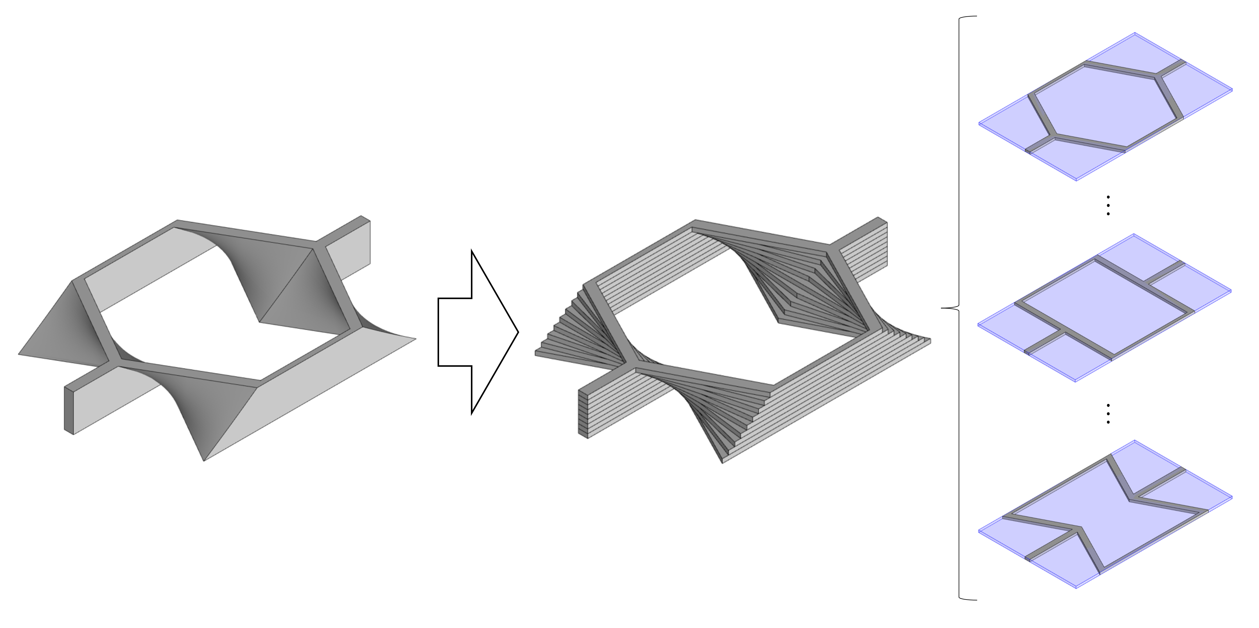
このように，対象形状を厚さ方向に複数層に分割し，それぞれの形状にたいして面内剛性行列を算出することでシェル要素の剛性行列を算出することが可能となります。 また，横せん断剛性は各層の足し合わせで算出します。

K_{ij} = \sum_{k=1}^{N}K_{ij}^{(k)}

面内剛性の算出

押出し形状の面内剛性は2次元有限要素解析により算出することができます。今回の対象形状は直交異方性を示すため，各方向のヤング率とポアソン比をE_L，E_T，ν_{LT}，ν_{TL}，横弾性係数をG_{LT}とすると，平面応力状態における単位長さあたりの荷重-変位関係は次のように表されます。

\begin{bmatrix} \sigma \end{bmatrix}
=
\begin{bmatrix} Q \end{bmatrix}
\begin{bmatrix} 
\varepsilon \end{bmatrix}\\
\begin{bmatrix} 
\sigma_L \\ \sigma_T \\ \tau_{LT}
\end{bmatrix}
=
\begin{bmatrix} 
\frac{E_L}{1-\nu_{LT}\nu_{TL}} &
\frac{\nu_{LT}E_T}{1-\nu_{LT}\nu_{TL}} & 0 \\
\frac{\nu_{TL}E_L}{1-\nu_{LT}\nu_{TL}} &
\frac{E_T}{1-\nu_{LT}\nu_{TL}} &
0\\
0&0&G_{LT}
\end{bmatrix}
\begin{bmatrix} 
\varepsilon_{L} \\ \varepsilon_{T}\\ \gamma_{LT}
\end{bmatrix}

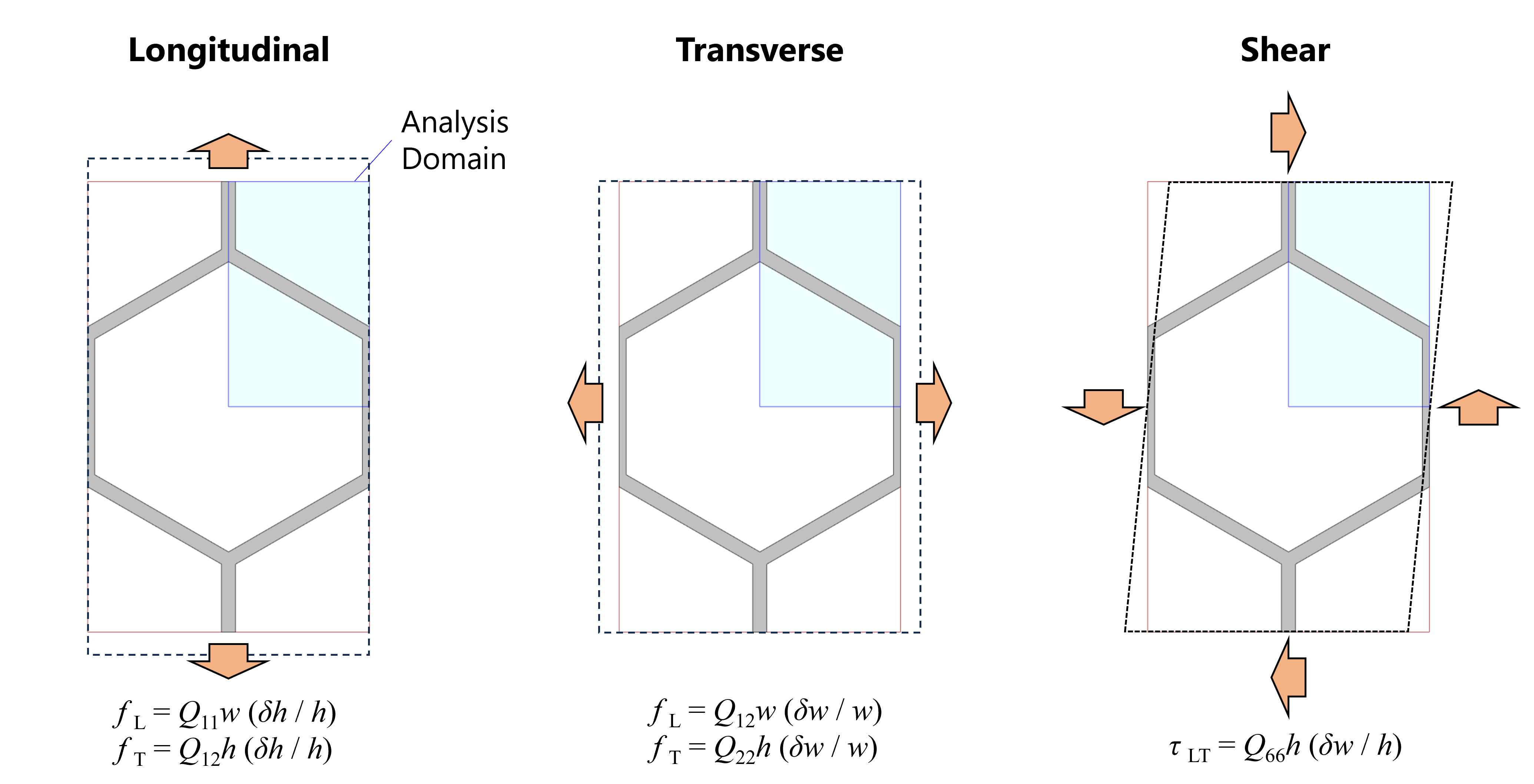
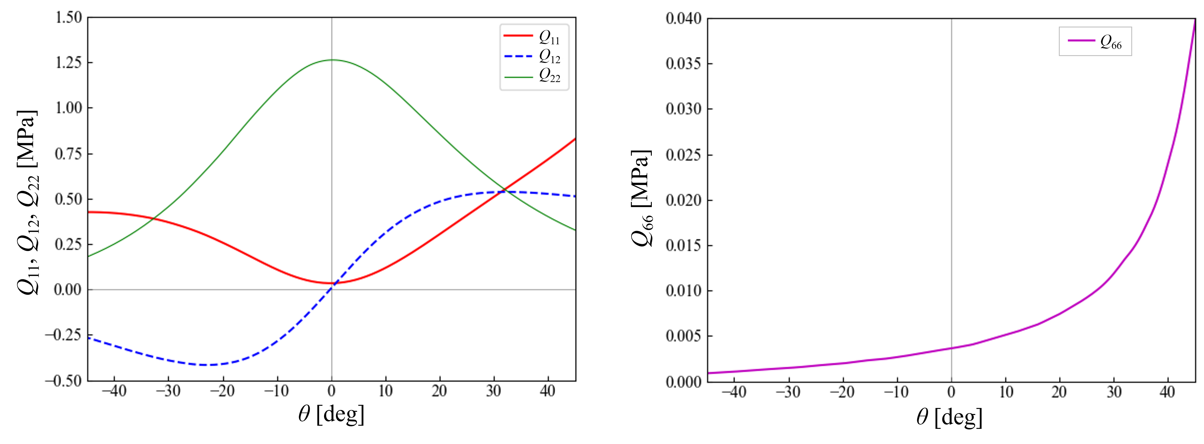
単位構造に対して，L方向，T方向，せん断の3つの強制変位条件で解析し，得られた反力をもとに剛性マトリクスの各成分を算出します。なお，計算時は対称境界または反対称境界を利用し，1/4モデルを用いました。 h = 1.6w, t_h = t_s = 0.05wとし，角度θを変化させたときの面内剛性行列の各成分は次のようになります。 これらの結果をもとに対象のメタマテリアルの特性を求めます。

シェル要素での解析

面内剛性が算出できたので，シェル要素の剛性行列を算出し有限要素解析をします。

要素剛性行列

今回の形状では，z=-t/2, t/2における梁の角度をθ_1, θ_2としたとき，板厚zにおける梁の角度θを次で表します。

\theta = \arctan{\left(
\frac{t/2-z}{t}\tan\theta_1 + \frac{z-t/2}{t}\tan\theta_2\right)}

t=2 {\text{mm}}とし，θ_1=30°，θ_2=30°とします。単位構造を30層に分割し，古典積層理論により算出した剛性行列は次のようになりました。

\begin{bmatrix} 
[A] & [B] \\ [B] & [D]
\end{bmatrix}
= \begin{bmatrix} 
0.435 \text{ N/mm} & 0.060 \text{ N/mm} & 0 & 0.032 \text{ N} & 0.419 \text{ N}& 0 \\
 & 1.850 \text{ N/mm} & 0 & 0.419 \text{ N}& 0.049\text{ N}& 0\\
 &  & 0.009\text{ N/mm} & 0 & 0 & 0.003\text{ N} \\
 & & & 0.221\text{ Nmm} & 0.032 \text{ Nmm}& 0\\
 & \text{sym.}& & & 0.477 \text{ Nmm}& 0\\
 & & & & & 0.004 \text{ Nmm}\\
\end{bmatrix}\\
\begin{bmatrix} 
[K]
\end{bmatrix}
=
\begin{bmatrix} 
1.552 \text{ N/mm} & 0\\
0 & 1.552\text{ N/mm}
\end{bmatrix}

なお，各層の横せん断剛性は面積比で近似しました。

a_{44} = a_{55} = Gt\times（単位構造の断面積）/wh

また，剛性行列の逆行列によって求められるコンプライアンス行列[S]を用いると，X方向荷重N_xによりY方向の曲率\kappa_yが発生することが分かります。

\begin{bmatrix} 
[\varepsilon] \\ [\kappa]
\end{bmatrix}=
\begin{bmatrix} [S] \end{bmatrix}
\begin{bmatrix} [N] \\ [M] \end{bmatrix}\\
\begin{bmatrix} 
\varepsilon_{x} \\ \varepsilon_{x}\\ \gamma_{xy}\\
\kappa_{x} \\ \kappa_{y} \\ \kappa_{xy}
\end{bmatrix}=
\begin{bmatrix} 
15.07\text{ mm/N}\\
-0.14\text{ mm/N}\\
 0 \\
0.03\text{ N}^{-1}\\
13.22\text{ N}^{-1}\\
0 \\
\end{bmatrix}
N_x

有限要素解析

ソリッド要素とシェル要素で解析を行い，結果を比較します。計算時には，材料非線形は考慮しませんが，幾何非線形は考慮します。

図のような形状に対して端をL方向に変位させたとき，反力および面外方向の変位の結果は次のようになりました。

• ソリッド：反力 9.38×10^{-2} \text N，面外方向変位 13.14 \text {mm}
• シェル：反力 8.24×10^{-2} \text N，面外方向変位 13.54 \text {mm}

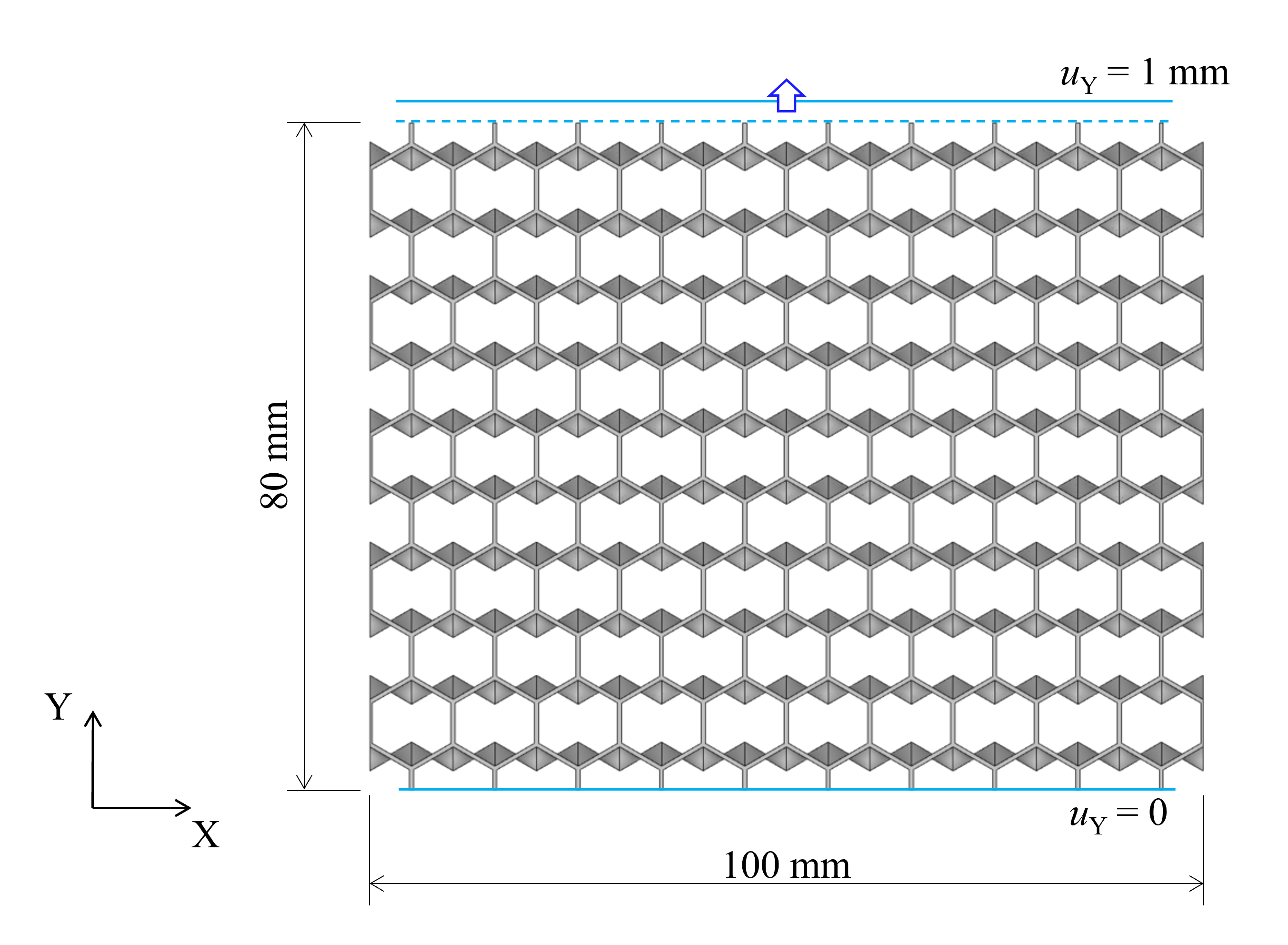
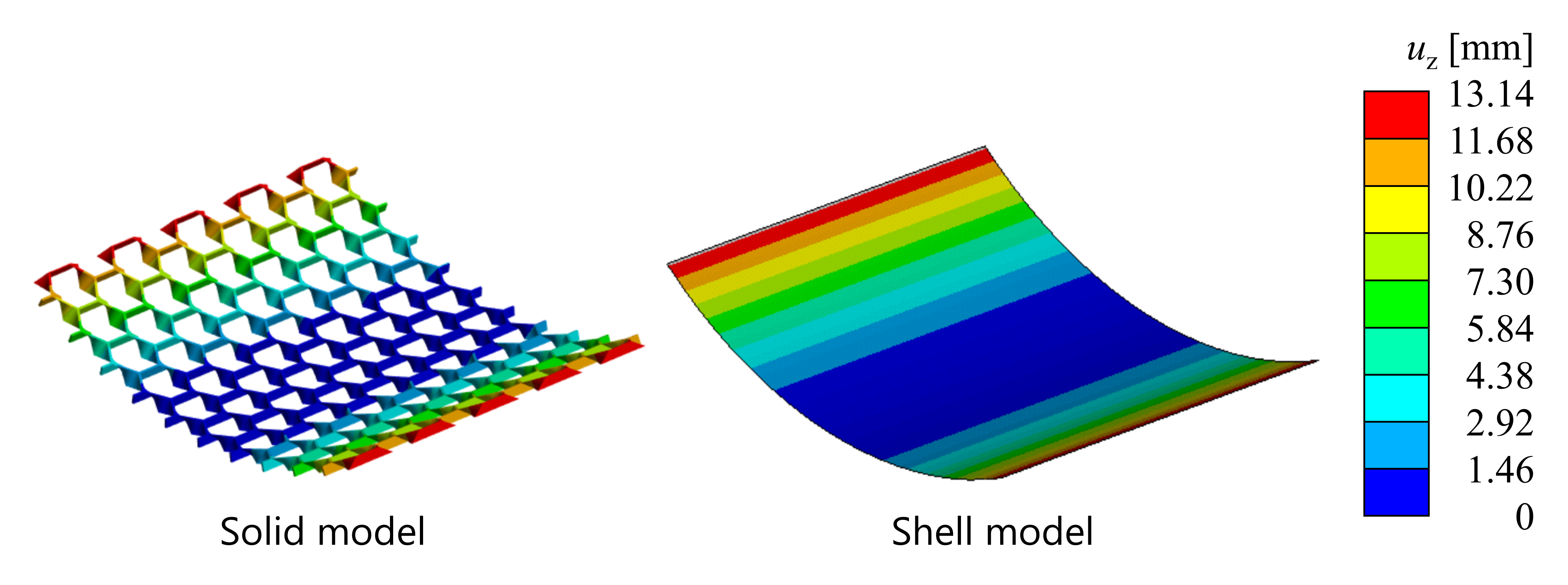
大まかな挙動を把握するには十分に近い値が得られています。 ここで生じた誤差の要因として,次が考えられます。

• すべての位置において中立面が板厚中央という前提のもとでシェル要素の剛性行列を算出したが，実際は中立面と中央面は一致しない。
• ソリッド要素の解析におけるメッシュ精度が十分でない。

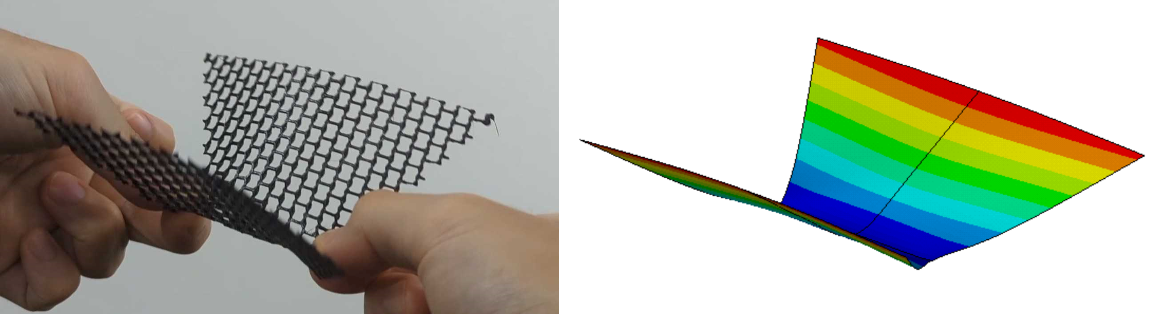
上では単純なケースを示しましたが，境界条件や形状が変わっても計算できます。本メタマテリアルで下図の蝶のような形状を作り，中央部を変位させた際の挙動を確認します。計算時は1/4モデルを使用しました。なお，ソリッド要素の解析は，収束性を考慮すると膨大な計算時間となってしまい，本形状では実施できませんでした。

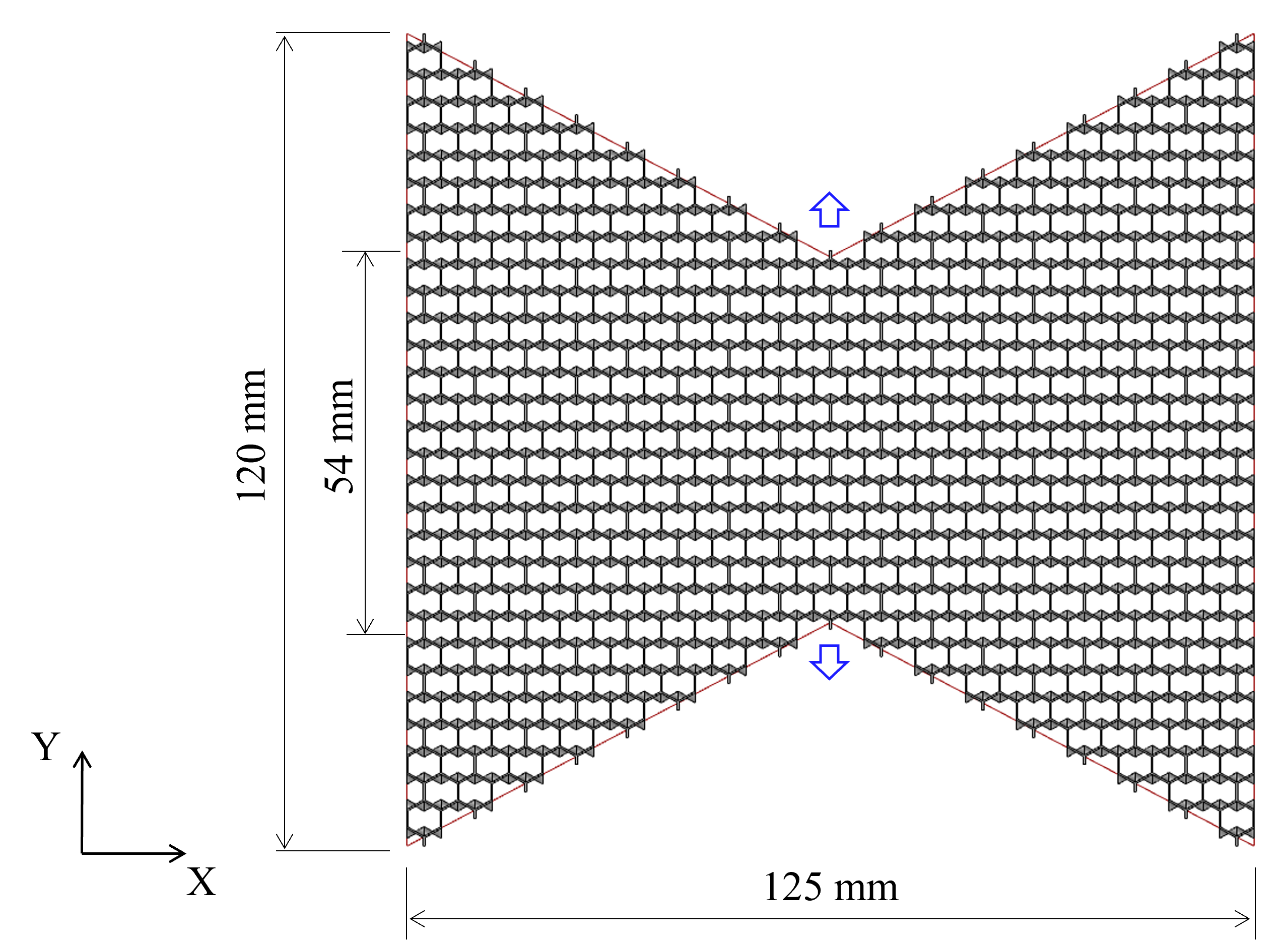
試作物に引張負荷をかけた際の概形は，シェル要素で解析した結果と類似しており，変形挙動を計算できていることが分かります。

まとめ

面内荷重によって面外変形を起こす機能を持つメタマテリアル構造の変形挙動を把握するため，有限要素解析を実施しました。

シェル要素を用いて均質化することで，変形挙動を簡易的にシミュレーションできることを示しました。また，シェル要素の剛性行列算出は，古典積層理論を用いることで2次元解析結果から近似できることを示しました。

References

- Imperial College London. Shell metamaterials. (Ref. Sep. 2023)