
はじめに
「有限要素法 (Finite Element Method, FEM)」と聞くと、機械設計に関心のある方であれば、構造解析を思い浮かべる方が多いと思います。中には、「有限要素法=構造解析の計算手法」と考えている方もいるかもしれません。しかしながら、有限要素法とはあくまで偏微分方程式を離散的に解く方法の一つですので、数値流体力学(Computational Fluid Dynamics, CFD)や電磁界解析など、構造解析以外の計算にも適用可能です。
同じく偏微分方程式を離散的に解く方法には、有限要素法の他にも、有限差分法 (Finite Difference Method, FDM)や有限体積法(Finite Volume Method, FVM)などといった手法があります。特に、有限体積法は商用・非商用問わず今日の実用的な流体解析ソルバーにおいては最も広く用いられる手法です。では、なぜ構造解析では有限要素法が主に用いられるのに対して、CFDでは有限体積法が広く用いられているのでしょうか。
実は、CFDにおいてどちらの方法が優れているのかは結論がついているものではなく、有限要素法のCFDへの適用については今でも世界中で日夜研究が行われています。そのため現在では、多くの場合、有限体積法を採用する理由は「既存の資産(先人の文献やプログラムなど)を利用したいから」「コミュニティが大きいから」等の人的な理由になるのかもしれませんが、CFD黎明期から有限体積法を選ぶ方向の潮流が生まれたのには何か別の理由があったはずです。
本記事では、CFDにおける有限要素法と有限体積法の基本的な定式を比較して「なぜCFDでは有限体積法が一般的になったのか」の理由を垣間見ていきます。
式の比較
以下の式で表される、1次元の偏微分方程式を考えます。
\(\tag{1}\frac{\partial\phi}{\partial t}+\frac{\partial f}{\partial x}=0\)
ここで\(\phi=\phi(t,x)\)は物理量、\(t\)は時間、\(x\)は座標、\(f=f(\phi)\)は流束を表しています。
有限要素法の定式
この式を有限要素法で解くには、任意の重み関数\(w(x)\)を掛けた上で計算領域\(\Omega\)全体で積分を行います。
\(\tag{2}\int_\Omega w(x)\left(\frac{\partial\phi^n}{\partial t}+\frac{\partial f^n}{\partial x}\right)dx=0\)
上付き文字の\(n\)はステップ数を表しています。有限要素法では、基底関数\(N(x)\)を用いて要素内の物理量の分布を補間します。
\(\tag{3}w(x)=N_i(x)w_i \\
\phi^n(x)=N_j(x)\phi_j^n\)
ここで\(i,j\)は要素番号で、アインシュタインの総和規約を適用しています。これらの式を起点として支配方程式の定式化を行います[1]。基底関数により要素内の物理量の分布を補間する部分が有限要素法の大きな特徴の一つです。その基底関数\(N(x)\)は多項式を用いるのが一般的ですが、その多項式の次数を増やすことで、高次の補間の定式化を行うことが有限体積法よりも容易にできます。
有限体積法の定式
一方、有限体積法では、重み関数を掛けずに式(1)を各計算セル(要素)\(\!^1\) 内で積分します\(\,^2\)。
\(\tag{4}\int_{\Omega_i} \frac{\partial\bar\phi_i^n}{\partial t}dx_i+\int_{\Omega_i}\frac{\partial f_i^n}{\partial x}dx_i=0\)
有限体積法では基本的には解をある点における値ではなくセル内の平均値として定義するため、平均値を表すバー(‾)を\(\phi\)につけています。左辺第二項をガウスの発散定理により境界積分に書き直すことで、有限体積法で解くべき式は以下のようになります。
\(\tag{5}\int_{\Omega_i} \frac{\partial\bar\phi^n_i}{\partial t}dx_i+\int_{\Gamma_i} \tilde f_i^n ds_i=0\)
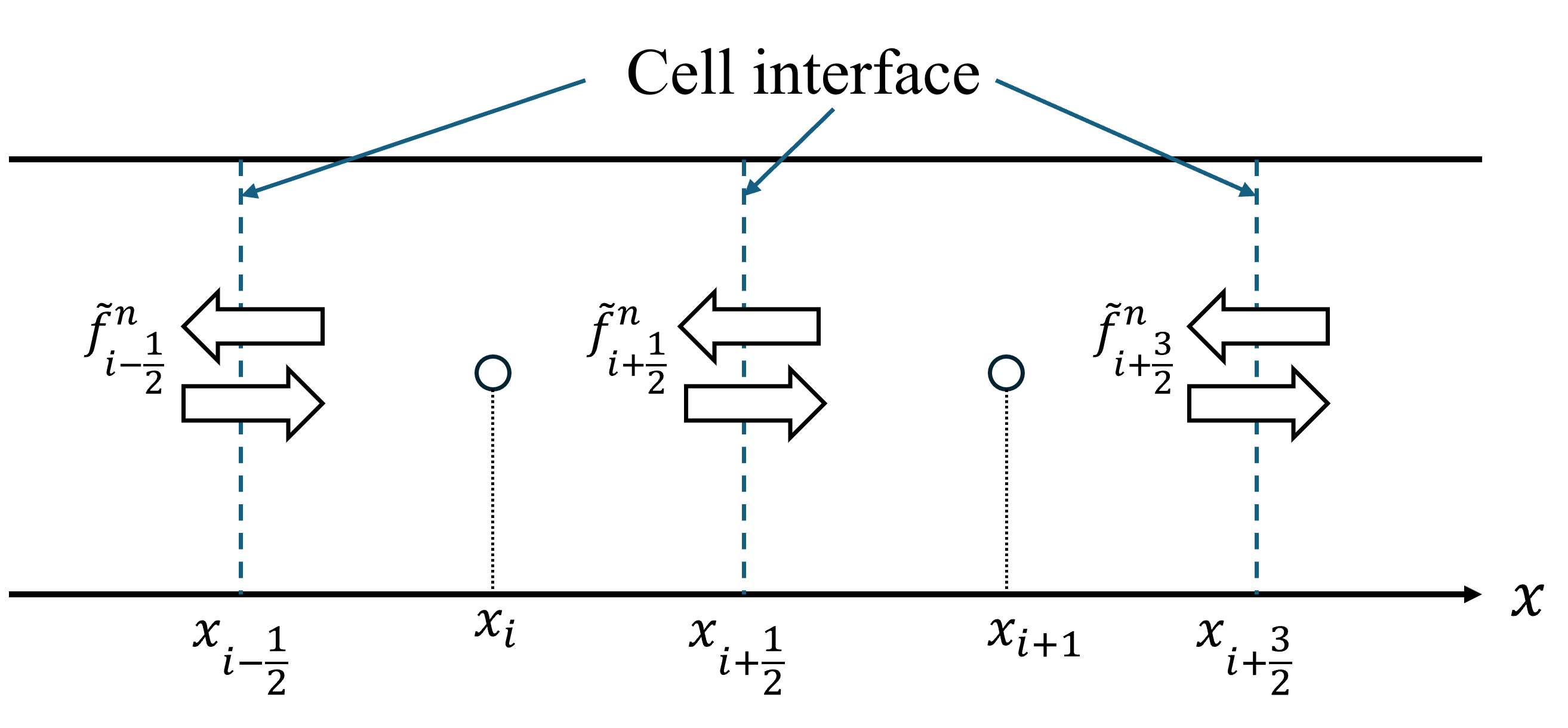
\(\tilde f\)はセル界面を通る流束である数値流束を表しています(セル代表点での流束である物理流束\(f\)とは区別してチルダを付けています)。また、\(\Gamma_i\)はセル\(i\)の境界、\(ds_i\)はセル\(i\)の境界の単位法線ベクトルを表しています。この式は解\(\bar\phi^n\)の変化はセル界面を通る流れの出入り(流束)のみによって決まることを表しています(下図)。
あるセルから出る流れは隣接するセルに入る流れと大きさは等しく符号は逆になるため、式(5)の全てのセルの総和をとれば、各セル界面の流れの出入りがキャンセルしあうことで、結局式(5)は計算領域全体でも成り立つことになります。
\(\tag{6}\int_\Omega \frac{\partial\bar\phi^n}{\partial t}dx+\int_\Gamma \tilde f^n ds=0\)
有限要素法の式(2)は、計算領域全体で保存則が満たされると解釈できる一方で、有限体積法の場合は、式(5),(6)より計算領域全体だけでなく計算セル1つ1つにおいても保存則が成立します\(\,^3\)。すなわち、基本的には有限体積法は有限要素法よりもより厳しく保存則が守られることを意味しています\(\,^4\)。流体解析では支配方程式が(質量・運動量・エネルギーの)保存則そのものであることから、直感的には有限体積法を用いる方が自然な選択のように思えます(この感覚も有限体積法が好まれてきた理由の1つかもしれません)。個人的には、有限要素法よりも有限体積法の定式の方が物理的な解釈が容易なので、それも有限体積法の参入障壁を下げてコミュニティの拡大に寄与したのではないかと想像しています。
有限要素法と比べた時の有限体積法の大きな特徴の一つとして、有限体積法では各セル界面における流束(数値流束)を陽的に計算するという点が挙げられます。その計算方法には任意性があるのが有限体積法の難しい(そして面白い)ところであり、同時に利点になるところでもあります。
\(\,^1\) 節点に囲まれた領域を有限要素法では「要素」、有限体積法では「セル」と呼ぶことが一般的です。
\(\,^2\) 注目する要素内では\(w_i(x)=1\), その外では\(w_i(x)=0\)となる重み関数を掛けて計算領域全体で積分するという解釈もできます。すると、有限体積法は有限要素法のある特殊な場合であると言えます。
\(\,^3\) 離散化の方法によってはこの局所的・大域的な保存性は満たされなくなります。例えば非保存形式の支配方程式を離散化した場合[2]。
\(\,^4\) 局所の保存性が満たされないと、局所的に非物理的なソース項が生じて計算が不安定になる場合があります。
計算してみる
それでは、有限要素法と有限体積法の定式の違いがわかったところで、実際にそれらを用いて単純な流れを解いてみましょう。有限要素法と有限体積法の有意な比較をすることは容易ではないので、ここではそれぞれの性能の比較ではなく、両者別々にとりあげてそれぞれの手法にどのような利点があるのかに着目します。
有限要素法での計算
まずは有限要素法を扱います。支配方程式は以下に示す一次元移流拡散方程式とします。
\(\tag{7}\frac{\partial\phi}{\partial t}+c\frac{\partial\phi}{\partial x}=\alpha\frac{\partial^2\phi}{\partial x^2}\)
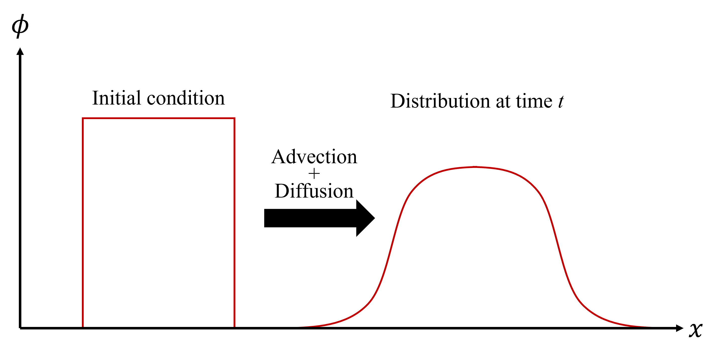
この式は下図のように物理量\(\phi\)の初期分布が速度\(c\)で移動しながら拡散係数\(\alpha\)で拡散していくことを表しています(\(c, \alpha\)は定数)。
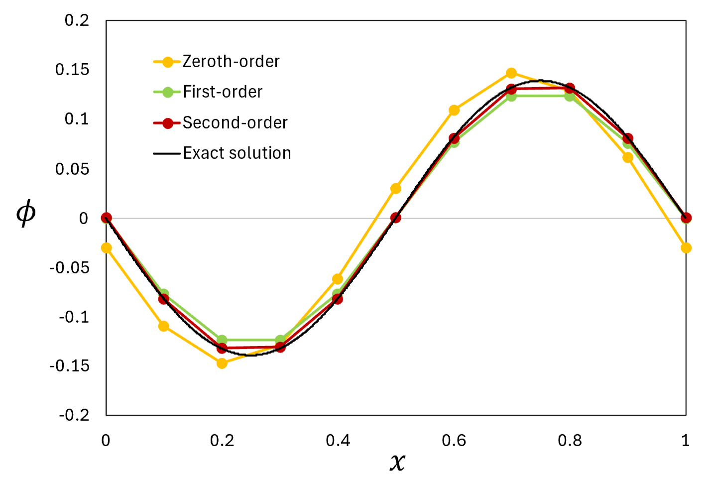
下図は物理量\(\phi\)の初期分布を\(\phi(x)=\mathrm{sin}(2\pi x)\quad(0\le x\le1)\)として、周期境界条件の下で節点数11, \(c=1.0\), \(\alpha=0.1\), また時間刻み\(\Delta t=5.0\times10^{-5}\)で \(t=0.5\)における解を0次(要素内一定)\(\,^1\)、1次(線形近似)、2次(二次曲線近似)補間を用いて求めた時の\(\phi\)分布です。
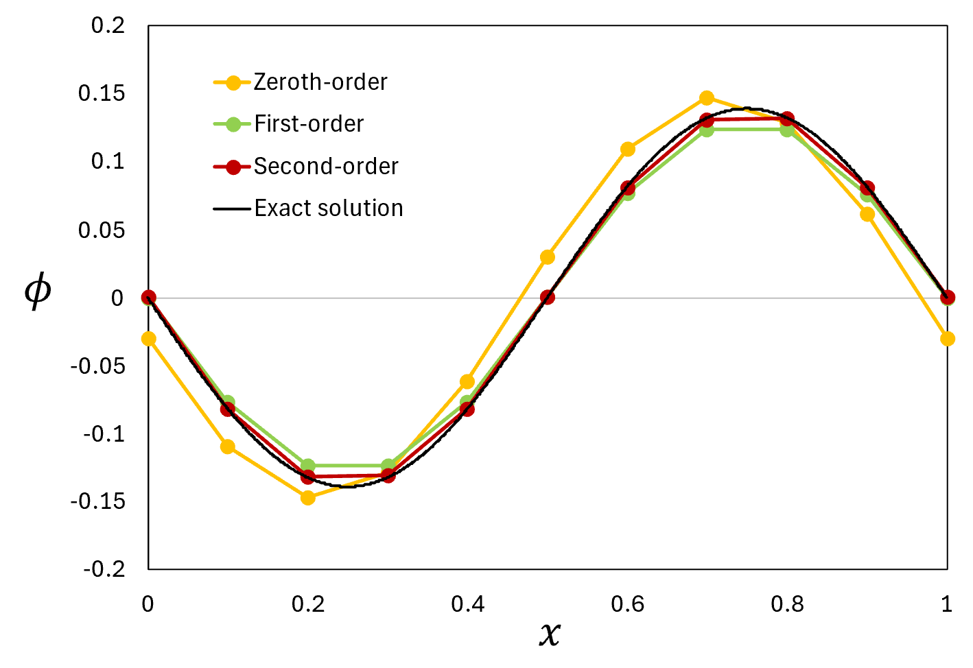
補間の次数が上がるとより解析解に近づく結果になりました。前述のように、有限要素法では要素内の物理量の分布を補間して計算を行います。その時に区分的多項式を用いて補間すると、多項式の次数を大きくすることで、2次補間よりもっと高次の定式化を行うことができます。有限体積法では精度の高い定式を作ることは有限要素法ほど容易ではないため、それが有限要素法の強みの1つと言えます。
有限体積法での計算
次に有限体積法を用いて流れを解きます。支配方程式は以下に示す一次元非粘性バーガース方程式とします。
\(\tag{8}\frac{\partial\phi}{\partial t}+\frac{\partial}{\partial x}\left(\frac{\phi^2}{2}\right)=0\)
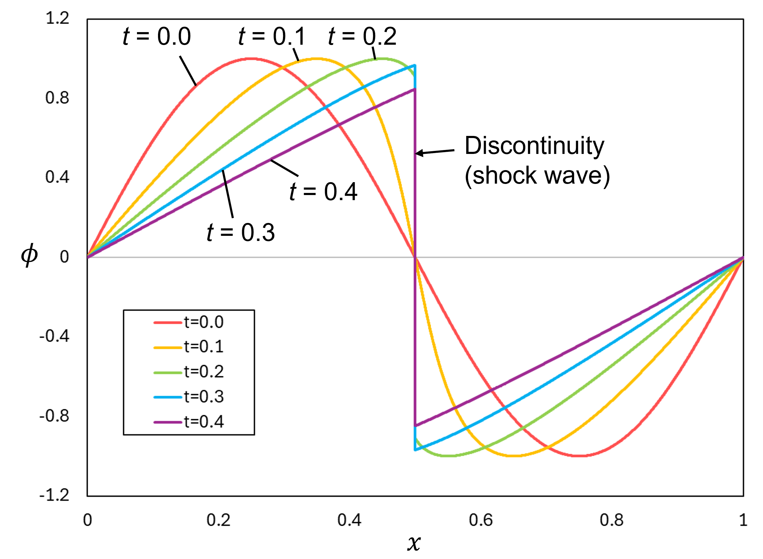
この式は物理量\(\phi\)の初期分布を\(\mathrm{sin}(2\pi x)\quad(0\le x\le1)\)とすると下図のように時間発展し、ある時刻以降に\(x=0.5\)に物理量\(\phi\)の不連続なジャンプ(衝撃波)を形成します。
前述のように、有限体積法では、セル界面の流束(数値流束)を計算しなければならず、その方法には任意性があります。例えばセル番号\(i\)と\(i+1\)の間の数値流束\(\tilde f_{i+\frac{1}{2}}\)を求める時、\(\tilde f_{i+\frac{1}{2}}=\tilde f(\frac{\bar\phi_i+\bar\phi_{i+1}}{2})\)としても\(\tilde f_{i+\frac{1}{2}}=\frac{f(\bar\phi_i)+f(\bar\phi_{i+1})}{2}\)としても解は得られます\(\,^2\)。また、これらのような算術平均に基づく定式ではなく、流れが来る上流側の物理量を用いて計算する風上法も以下のように容易に定式化できます。
\(\tag{9}\tilde f_{i+\frac{1}{2}}=\frac{1}{2}\left(\frac{\bar\phi_{i+1}^2}{2}+\frac{\bar\phi_i^2}{2}\right)-\left|\frac{(\bar\phi_{i+1}+\bar\phi_i)}{2}\right| \frac{(\bar\phi_{i+1}-\bar\phi_i)}{2}\)
この式は、\(\phi_{i+\frac{1}{2}}=\frac{(\bar\phi_{i+1}+\bar\phi_i)}{2}\gt0\)の時\(\tilde f_{i+\frac{1}{2}}=\frac{\bar\phi_i^2}{2}=f_i\)に、\(\phi_{i+\frac{1}{2}}\lt0\)の時\(\tilde f_{i+\frac{1}{2}}=f_{i+1}\)になります。これらの式を用いて、\(\phi(x)=\mathrm{sin}(2\pi x)\quad(0\le x\le1)\)を初期分布として節点数101かつ時間刻み\(\Delta t=1.0\times10^{-3}\)で\(t=0.2\)における流れを解いたものが下図になります。
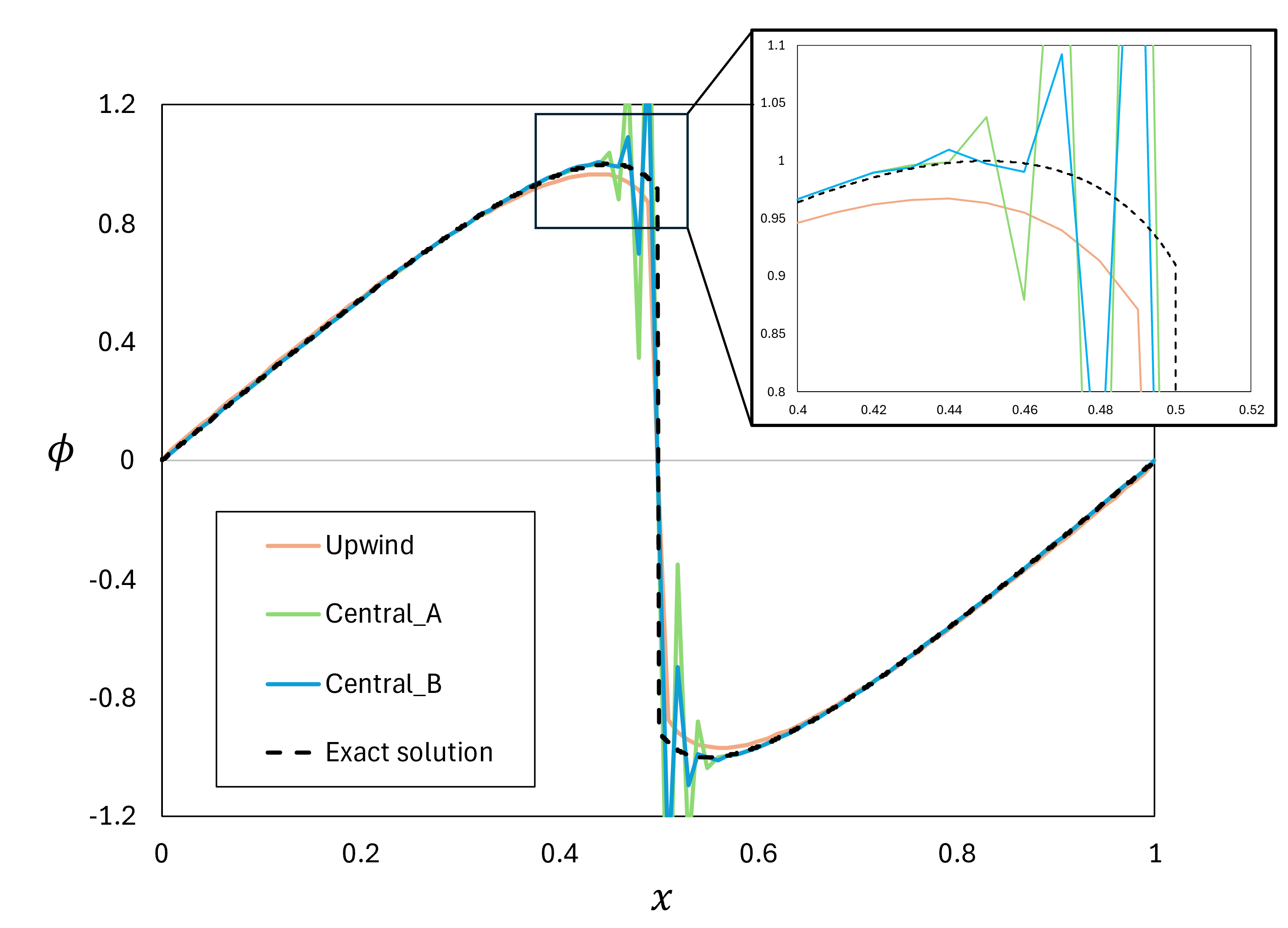
算術平均に基づく定式(Central_AとCentral_B)では物理量が急に変化する部分で振動が生じてしまいました。風上法では振動は無くなりましたが、解がなまってしまいました。詳細は省きますが、これは風上法では解をなまして計算を安定させる数値粘性が生じることに起因します。であれば、物理量が急激に変化する部分でのみ風上法になる計算手法があれば、計算精度を保った上で安定な計算ができるように思えますね。有限体積法では、そのようなアイデアを以下のように簡単に実現することができます(ただし、今回の問題設定では以下の説明で得られる定式は有限差分法と同一になります)。
風上法の式(9)をよく見ると、右辺第一項は物理流束\(f_{i+1}\)と\(f_i\)の算術平均(図5のCentral_Bと同一)であることから、第二項は実質的に数値粘性を含む項だと考えられます。そこで、局所の物理量の勾配に応じて数値粘性の大きさを変えられるように、以下のように第二項に制限関数\(L(r_{i+\frac{1}{2}})\)をかけてみます。
\(\tag{10}\tilde f_{i+\frac{1}{2}}=\frac{1}{2}\left(\frac{\bar\phi_{i+1}^2}{2}+\frac{\bar\phi_i^2}{2}\right)-L(r_{i+\frac{1}{2}})\left|\frac{(\bar\phi_{i+1}+\bar\phi_i)}{2}\right| \frac{(\bar\phi_{i+1}-\bar\phi_i)}{2}\)
ここで\(L(r_{i+\frac{1}{2}})\)は\(r_{i+\frac{1}{2}}=\frac{\phi_i-\phi_{i-1}}{\phi_{i+1}-\phi_i}\)の関数です。物理量が急激に変化する場所では\(L(r_{i+\frac{1}{2}})=1\)で風上法となり、物理量が滑らかに変化する場所では\(L(r_{i+\frac{1}{2}})=0\)で算術平均になるような関数を設定してみます。関数の中身には任意性がありますが、ここでは
\(\tag{11}L(r)=1-\mathrm{max}[0,\mathrm{min}(1,r)]\)
とします\(\,^3\)。この式を用いて同じ流れを解くと以下の図のようになります。
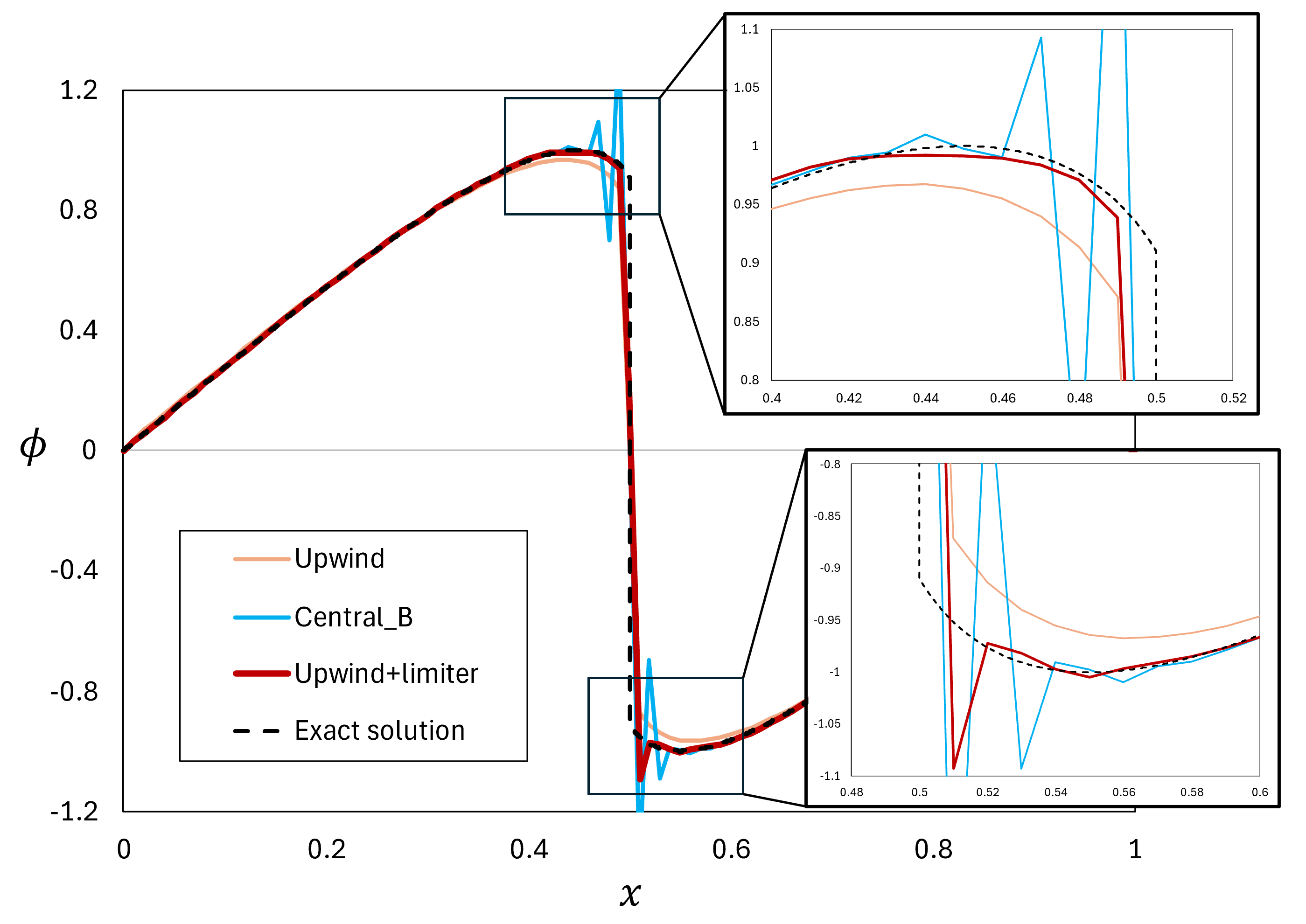
まだ\(x=0.52\)付近で振動は残っているものの、算術平均(Central_B)よりも振動が小さく、また風上法よりも高精度で流れを解くことができました。
以上の例のように、基本的な有限体積法のアルゴリズムでは、数値流束を陽に計算するため、局所の流れ場の情報を反映させた計算手法を組み込むことが容易にできます。流体の運動を表すNavier–Stokes方程式は非線形性が非常に強いので、計算領域内に局所的に生じた複雑な物理現象に対して安定に計算し続けられるような対処が実装上容易だったことが、有限体積法が有限要素法よりも好まれた理由の1つなのだと考えられます。そのようにして有限体積法のコミュニティが拡大したことが、CFDで有限体積法が一般的になる一助になったのではないでしょうか。
\(\,^1\) 1次補間で集中化質量行列を用いることに相当します。また今回の問題設定では、0次補間で得られる定式は、時間は一次精度前進差分法かつ空間は二次精度中心差分法で離散化した有限差分法・有限体積法と同じ定式になります。
\(\,^2\) 後者は有限差分法で二次精度中心差分法を用いた定式と同一になります。
\(\,^3\) 右辺第二項はminmod関数と言います。
おわりに
本記事では、有限要素法と有限体積法の基本的な定式・強みの違いを比較して、CFDで有限体積法が一般的になった理由の一端を探ってみました。
今回触れたのはあくまで有限体積法と有限要素法の違いの一部であり、またそれぞれのアルゴリズムの基本的(古典的)な部分のみを見てきました。現在では有限要素法・有限体積法共に発展し続けており、両手法がお互いの強みも持ち合わせた手法が提案されていたりと、CFDの計算手法の研究は止まるところを知りません。
前述のように、流体解析において有限要素法と有限体積法のどちらが優れているかは結論がついているものではなく、今後有限要素法が優勢になる可能性もありますし、やはり有限体積法が一般的であり続ける可能性もあります。もしかしたら両者でもなく別の計算手法が一般的になるかもしれません。いずれにしても、CFDを行う上では計算手法の中身を理解した上で、計算する対象の物理に合わせて適切な手法を選択することが重要です。
参考文献
[1] 河野晴彦,“詳解 流れの数値計算 - 有限要素法による非圧縮性流体解析の基礎 -”,コロナ社,2022,pp. 46–100.
[2] Hirsch, C., Numerical Computation of Internal and External Flows: The Fundamentals of Computational Fluid Dynamics, 2nd ed., Butterworth-Heinemann, 2007, pp. 206–208.
Introduction
When you hear the term “Finite Element Method (FEM),” if you are interested in mechanical design, probably many of you would imagine structural analyses. Some people may think that FEM is the calculation method only for structural analyses. However, FEM is just one of the methods to solve partial differential equations (PDEs) discretely and is applicable to not only structural analyses but also computational fluid dynamics (CFD), electromagnetic analyses, etc.
There are many methods for solving PDEs discretely other than FEM, such as finite difference method (FDM) and finite volume method (FVM). Particularly, FVM is the most common method in today’s practical commercial/non-commercial fluid analysis solvers. But why is FVM common in CFD whereas FEM is usually adopted in structural analyses?
Actually, the question whether FEM or FVM is more appropriate for CFD does not still reach a conclusion, and research on FEM to apply to CFD is ongoing around the world. Therefore, today’s reasons for adopting FVM in CFD may be “because we want to utilize existing assets (literature or programs of predecessors)” or “because the FVM community is bigger than the FEM community” and not based on their innate physics. However, there must have been other reasons for that the trend toward choosing FVM was born in the early days of CFD.
This article compares basic formulations of FEM and FVM in CFD and catches a glimpse into the reasons “why FVM become the common method in CFD.”
Comparison of formulations
Consider the following one-dimensional (1D) PDE:
\(\tag{1}\frac{\partial\phi}{\partial t}+\frac{\partial f}{\partial x}=0\)
where \(\phi=\phi(t,x)\) is a physical quantity, \(t\) is time, \(x\) is coordinate, and \(f=f(\phi)\) is flux.
Formulation of finite element method
To solve this PDE using FEM, we integrate Eq. (1) over computational domain \(\Omega\) after multiplying arbitrary weight function \(w(x)\).
\(\tag{2}\int_\Omega w(x)\left(\frac{\partial\phi^n}{\partial t}+\frac{\partial f^n}{\partial x}\right)dx=0\)
where the superscript \(n\) denotes time step. In FEM, distributions of a physical quantity in each element are interpolated by using the basis function \(N(x)\).
\(\tag{3}w(x)=N_i(x)w_i \\
\phi^n(x)=N_j(x)\phi_j^n\)
where \(i\) and \(j\) denote element numbers, and the Einstein summation convention is applied. These equations are used as the starting point to obtain the governing equation in FEM [1]. This interpolation using the basis functions is one of the main characteristics of FEM. The basis function usually uses a polynomial, and by increasing the order of the polynomial, it is easier than FVM for FEM to obtain higher-order interpolation formulations.
Formulation of finite volume method
On the other hand, FVM integrates Eq. (1) over each computational cell\(\,^1\) without multiplying the weight function\(\,^2\).
\(\tag{4}\int_{\Omega_i} \frac{\partial\bar\phi_i^n}{\partial t}dx_i+\int_{\Omega_i}\frac{\partial f_i^n}{\partial x}dx_i=0\)
Because FVM defines solutions as an averaged value in each cell rather than values at some points, Eq. (4) has bars (‾), which indicate an averaged value, over \(\phi\). By rewriting the second term on the left-hand side into boundary integral using Gauss’ divergence theorem, the equation solved in FVM is obtained as follows:
\(\tag{5}\int_{\Omega_i} \frac{\partial\bar\phi^n_i}{\partial t}dx_i+\int_{\Gamma_i} \tilde f_i^n ds_i=0\)
\(\tilde f\) is the numerical flux, which is flux through cell interfaces (tilde differentiates numerical flux from physical flux \(f\), which is flux at a representative point in a cell). \(\Gamma_i\) is the boundary of cell \(i\), and \(ds_i\) is the unit normal vector of the boundary of cell \(i\). This equation means the changes in solution \(\bar\phi^n\) depend only on the inflow and outflow (flux) at the cell interface (figure below).
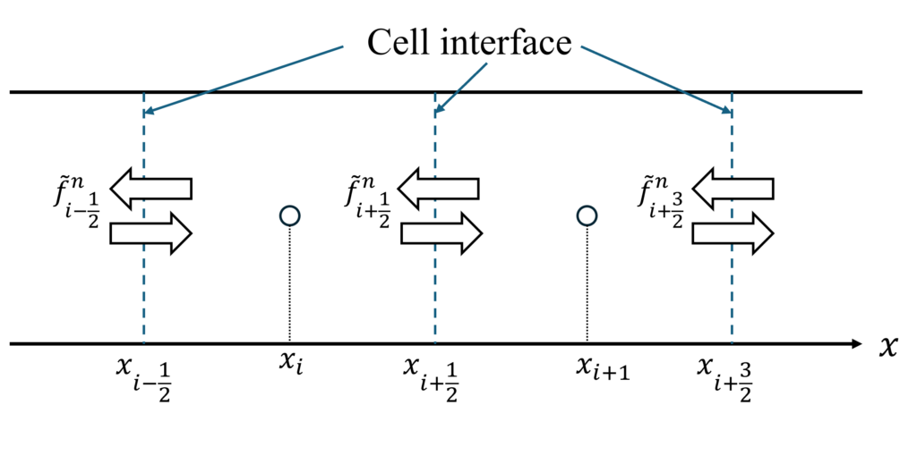
Fig. 1 Schema of equation (5).
Because outflow from a cell is inflow to the next cell with the same magnitude and opposite sign, summing Eq. (5) over all cells leads to the following equation:
\(\tag{6}\int_\Omega \frac{\partial\bar\phi^n}{\partial t}dx+\int_\Gamma \tilde f^n ds=0\)
This equation shows that Eq. (5) also holds for the entire computational domain. Whereas Eq. (2) of FEM can be interpreted as that the conservation law is satisfied over the entire domain, Eqs. (5) and (6) of FVM show that the conservation law is satisfied over not only the entire domain but also each cell\(\,^3\). That is, basically the conservation law is more strictly kept in FVM than FEM\(\,^4\). Because fluid calculations employ the conservation laws (of mass, momentum, and energy) itself as its governing equations, using FVM in CFD feels like a natural choice (and this intuition may be one of the reasons why FVM has been widely accepted). In my view, because the formulation of FVM is easier for physical interpretation than that of FEM, I suspect this easiness to understand also led to an expansion of the FVM community.
One of the main characteristics of FVM in comparison with FEM is that FVM explicitly calculates flux at each cell interface (numerical flux). The arbitrariness of the way of the calculation is a difficult (and interesting) point but also an advantageous point in FVM.
\(\,^1\) a region surrounded by nodes is commonly called “element” in FEM and “cell” in FVM.
\(\,^2\) It is possible to interpret the formulation as integrated over the entire domain with multiplying a weight function that becomes $w_i(x)=1$ in a cell of interest and $w_i(x)=0$ outside the cell. Then, FVM can be considered as a special case of FEM.
\(\,^3\) This local and global conservation property is not necessarily held. For example, when governing equations in non-conservation form are discretized [2].
\(\,^4\) If local conservation is not satisfied, a local unphysical source term arises and the calculation can become unstable in some cases.
Calculations
Now that we know the difference between the formulations of FEM and FVM, let’s actually solve simple flows using them. Because it is difficult to fairly compare FEM and FVM, here we will not compare their performance but rather focus on their advantages by taking them separately.
Calculations using finite element method
First, we focus on FEM. A governing equation is the following 1D advection–diffusion equation:
\(\tag{7}\frac{\partial\phi}{\partial t}+c\frac{\partial\phi}{\partial x}=\alpha\frac{\partial^2\phi}{\partial x^2}\)
This equation means an initial condition of the physical quantity \(\phi\) moves with velocity \(c\) while diffusing with diffusion coefficient \(\alpha\) (\(c\) and \(\alpha\) are constants) as in the following figure.
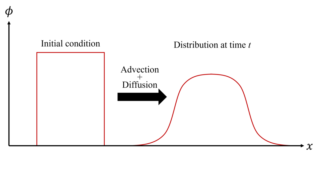
Fig. 2 Schema of advection–diffusion equation.
The next figure shows the calculated results of advection–diffusion equation with \(\phi(x)=\mathrm{sin}(2\pi x)\quad(0\le x\le1)\) as the initial distribution and periodic boundary condition. The solutions were obtained using zeroth-order (constant within an element)\(\,^1\), first-order (linear approximation), and second-order (quadratic approximation) interpolation at \(t=0.5\) with 11 nodes, \(c=1.0\), \(\alpha=0.1\), and time step \(\Delta t=5.0\times10^{-5}\).

Fig. 3 Calculated results of advection–diffusion equation with \(\phi(x)=\mathrm{sin}(2\pi x)\quad(0\le x\le1)\) as the initial distribution using FEM (t=0.5).
This figure shows the calculated solutions approach to the analytical solution as the order of interpolation increases. As mentioned before, FEM calculates solutions while interpolating the distribution of physical quantity within elements. If piecewise polynomials are employed in the interpolation, we can obtain higher-order (than second-order) formulations by increasing the order of the polynomial. Because obtaining formulations of high accuracy in FVM is not as easy as in FEM, this point is one of the advantages of FEM.
Calculations using finite volume method
Next, we solve flows using FVM. A governing equation is following 1D inviscid Burgers’ equation:
\(\tag{8}\frac{\partial\phi}{\partial t}+\frac{\partial}{\partial x}\left(\frac{\phi^2}{2}\right)=0\)
This equation evolves in time as shown in the following figure when the initial condition of the physical quantity \(\phi\) is \(\phi(x)=\mathrm{sin}(2\pi x)\quad(0\le x\le1)\), and a discontinuous jump of \(\phi\) (shock wave) is formed at \(x=0.5\) after a certain time.
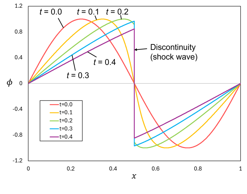
Fig. 4 Time evolution of inviscid Burges equation with initial distribution of \(\phi(x)=\mathrm{sin}(2\pi x)\).
As mentioned before, FVM needs to calculate flux at each cell interface (numerical flux), and its means have arbitrariness. For example, when we calculate a numerical flux \(\tilde f_{i+\frac{1}{2}}\) that is midpoint of cell number \(i\) and \(j\), we can obtain solution by defining it as \(\tilde f_{i+\frac{1}{2}}=\tilde f(\frac{\bar\phi_i+\bar\phi_{i+1}}{2})\), \(\tilde f_{i+\frac{1}{2}}=\frac{f(\bar\phi_i)+f(\bar\phi_{i+1})}{2}\), etc\(\,^2\). Additionally, rather than the formulations based on arithmetic averages like these, we can easily obtain an upwind scheme that calculates numerical flux using physical quantity from upstream cells as follows:
\(\tag{9}\tilde f_{i+\frac{1}{2}}=\frac{1}{2}\left(\frac{\bar\phi_{i+1}^2}{2}+\frac{\bar\phi_i^2}{2}\right)-\left|\frac{(\bar\phi_{i+1}+\bar\phi_i)}{2}\right| \frac{(\bar\phi_{i+1}-\bar\phi_i)}{2}\)
This equation means that \(\tilde f_{i+\frac{1}{2}}=\frac{\bar\phi_i^2}{2}=f_i\) when \(\phi_{i+\frac{1}{2}}=\frac{(\bar\phi_{i+1}+\bar\phi_i)}{2}\gt0\) and \(\tilde f_{i+\frac{1}{2}}=f_{i+1}\) when \(\phi_{i+\frac{1}{2}}\lt0\). The following figure shows the calculated results at \(t=0.2\) using the above equations with \(\phi(x)=\mathrm{sin}(2\pi x)\quad(0\le x\le1)\) as initial distribution, 101 nodes, and time step \(\Delta t=1.0\times10^{-3}\).

Fig. 5 Calculated results of Burgers’ equation using FVM (t = 0.2). Upwind means an upwind scheme, Central_A means \(\tilde f_{i+\frac{1}{2}}=\tilde f((\bar\phi_i+\bar\phi_{i+1})/2)\), and Central_B menas \(\tilde f_{i+\frac{1}{2}}=(f(\bar\phi_i)+f(\bar\phi_{i+1}))/2\).
The formulations based on arithmetic averages (Central_A and Central_B) caused oscillation near the discontinuity where the physical quantity changed abruptly. Although Upwind does not cause oscillation, the solution became somewhat diffusive. I will not go into details, but this is because the upwind method produces numerical viscosity, which diffuses a solution and stabilizes calculation. Then, if there is a calculation method that becomes an upwind scheme only where the physical quantity changes sharply, it seems the calculation is stable while maintaining accuracy. In FVM, this idea can be easily implemented as follows (the formulation obtained in the following explanation is the same as FDM in this problem setting).
A closer look at Eq. (9) of the upwind scheme shows that the first term of the right-hand side is the arithmetic average of the physical flux \(f_{i+1}\) and \(f_i\) (same as Central_B), so the second term is effectively a term involving numerical viscosity. So that the magnitude of the numerical viscosity can be changed in response to the local gradient of the physical quantity, we apply a limiting function \(L(r_{i+\frac{1}{2}})\) to the second term as follows:
\(\tag{10}\tilde f_{i+\frac{1}{2}}=\frac{1}{2}\left(\frac{\bar\phi_{i+1}^2}{2}+\frac{\bar\phi_i^2}{2}\right)-L(r_{i+\frac{1}{2}})\left|\frac{(\bar\phi_{i+1}+\bar\phi_i)}{2}\right| \frac{(\bar\phi_{i+1}-\bar\phi_i)}{2}\)
where \(L(r_{i+\frac{1}{2}})\) is the function of \(r_{i+\frac{1}{2}}=\frac{\phi_i-\phi_{i-1}}{\phi_{i+1}-\phi_i}\). We define the function such that \(L(r_{i+\frac{1}{2}})=1\) and becomes the upwind scheme where the physical quantity changes rapidly and \(L(r_{i+\frac{1}{2}})=0\) and becomes arithmetic average where the physical quantity changes smoothly. The function has arbitrariness, but here we define it as\(\,^3\)
\(\tag{11}L(r)=1-\mathrm{max}[0,\mathrm{min}(1,r)]\)
The following figure shows the calculated results using these equations.

Fig. 6 Calculated results of inviscid Burgers’ equation using FVM (t = 0.2). Upwind+limiter has the formulations of Eqs. (10) and (11).
Although oscillation still remains near \(x=0.52\), the oscillation is smaller than the arithmetic average (Central_B), and the solution is closer to the analytical solution than that of the upwind scheme.
As shown in the above example, the basic FVM algorithm calculates numerical fluxes explicitly and therefore can easily implement calculation methods, which include local information of flow fields. Because the Navier–Stokes equation, which describes fluid motion, has strong non-linearity, the easiness of the implementation of special treatments for stabilization in response to complicated flow phenomena that arose locally could be one of the reasons for choosing FVM rather than FEM. It can be considered that the expansion of the FVM community in this way may have helped FVM become more common in CFD.
\(\,^1\) This is the same as using the lumped mass matrix in the first-order interpolation. Besides, in this problem setting, the formulation of zeroth-order interpolation is the same as the FDM and FVM that discretized with the first-order forward difference method in time and the second-order central difference method in space.
\(\,^2\) The latter is the same as the formulation of FDM with the second-order central difference method.
\(\,^3\) The second term on the right-hand side is called minmod function.
Conclusion
This article compared the basic formulations and advantages of FEM and FVM and investigated some reasons why FVM became common in CFD.
This time we discussed just some parts of the differences between FEM and FVM and looked at only the basic (classical) parts of them. Today, both FEM and FVM continue to develop, and methods that the two have each other’s strengths have been proposed.
As aforementioned, the question of whether FEM of FVM is better in CFD has not reached a conclusion. In the future, FEM may become common in CFD, or FVM may remain common. Perhaps another method will become common. In any case, when conducting CFD, it is important to understand the formulations of the calculation methods and then select an appropriate method according to the physics of the flow of interest.
Reference
[1] Kohno, H., Detailed Description of Numerical Methods in Fluids - Fundamentals of Finite Element Analysis of Incompressible Fluid Flows, Corona Publishing, 2022, pp. 46–100. (in Japanese)
[2] Hirsch, C., Numerical Computation of Internal and External Flows: The Fundamentals of Computational Fluid Dynamics, 2nd ed., Butterworth-Heinemann, 2007, pp. 206–208.
