
どんな最適化に向いているか
設定について考える前に、そもそも Tunny で使用可能な最適化手法そのものの得意不得意を確認します。
Tunny はたくさんの最適化手法に対応しているので、どれを選べばよいか悩むことがあります。
公式ページにあるそれぞれの得意不得意と、私が作成した選択のフローチャートをまず記載します。
| RandomSampler | TPESampler | CmaEsSampler | NSGAIISampler | GPSampler | BoTorchSampler | |
|---|---|---|---|---|---|---|
| Float parameters | ✓ | ✓ | ✓ | ▴ | ✓ | ✓ |
| Integer parameters | ✓ | ✓ | ✓ | ▴ | ✓ | ▴ |
| Categorical parameters | ✓ | ✓ | ▴ | ✓ | ✓ | ▴ |
| Pruning | ✓ | ✓ | ▴ | × | ▴ | ▴ |
| Multivariate optimization | ▴ | ✓ | ✓ | ▴ | ✓ | ✓ |
| Conditional search space | ✓ | ✓ | ▴ | ▴ | ▴ | ▴ |
| Multi-objective optimization | ✓ | ✓ | × | ✓ (▴ for single-objective) | × | ✓ |
| Batch optimization | ✓ | ✓ | ✓ | ✓ | ▴ | ✓ |
| Distributed optimization | ✓ | ✓ | ✓ | ✓ | ▴ | ✓ |
| Constrained optimization | × | ✓ | × | ✓ | × | ✓ |
| Recommended budgets (#trials) | as many as one likes | 100 – 1000 | 1000 – 10000 | 100 – 10000 | – 500 | 10 – 100 |
選択のフローチャート
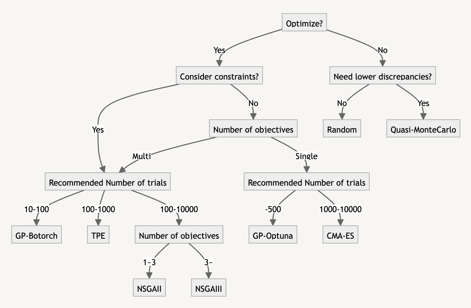
フローチャートはまずこれを試してみた方が良い程度の指標です。
実際に扱おうしている問題に必ずしもあっているとは限らないので、いろいろ試してみてください。
では実際に使ってみたときの挙動を見てみましょう。
Tunny のデフォルトでの最適化
Tunny は他の最適化プラグインと異なり、デフォルトの最適化の手法は GA ではなく TPE になっています。
またいろいろな手法がサポートされています。
あまり馴染みがない方も多いと思いますので、ここでは設定を何もいじらずデフォルトで動作させたときにどうなるか見てみましょう。
最適化の手法を確認する際には色々なベンチマーク関数を使用しますが、そんなことは考えずにただの2つの NumberSlider の和の最小化問題を解いてみましょう。
0~1 の範囲で値を取る NumberSlider ですが、小数点以下 1/10,000 まであります。
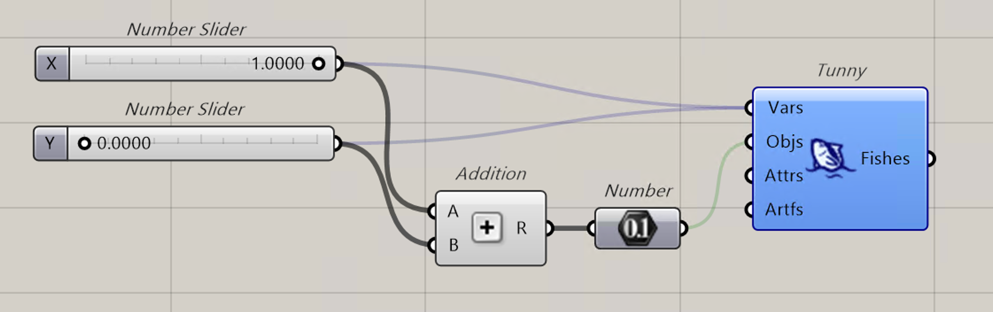
本記事ではA+Bを対象にしていますが、ベンチマーク関数次第で最適化の優劣が変わることが知られています。
そのため、本記事での検討は設定が最適化に与える影響の一例として考えてください。
TPE を使った最適化
では何も考えずに Tunny のデフォルトの設定で最適化を実行してみます。
デフォルトでは以下になっています。
- 試行回数:100
TPE の設定
- seed : 自動計算
- 疑似乱数を生成するアルゴリズムのシード
- Number of startup trials : 10
- TPE で探索する前のランダムサンプリングでの初期化の試行数
- Number of EI candidates : 24
- 獲得関数を評価する際に使用するサンプリング数
- Consider Prior : True
- 探索と活用のトレードオフにおいて探索の比重を高める関数の有効化
- Prior weight : 1.0
- 上記関数の重み
- Consider Endpoints : False
- True のとき変数の両端を丁寧に探索する
- Consider Magic Clip : True
- 最適化計算で使用する分散の値の下限値の有効化
- Multivariate : False
- 多変量 TPE の有効化
- Group : False
- Multivariate が True のときに探索空間をいくつかの Group に分割した探索の有効化
- Constant Liar : False
- 分散並列最適化の効率を上げる Constant Liar アルゴリズムの有効化
最適化は一部で疑似乱数を使っており、実行するたびに結果が変わるので、5 回最適化を実行しています。
なお疑似乱数を生成するシード値を直接指定することもできるため、最適化の再現を行うこともでき、あとの章でこの機能を使っています。
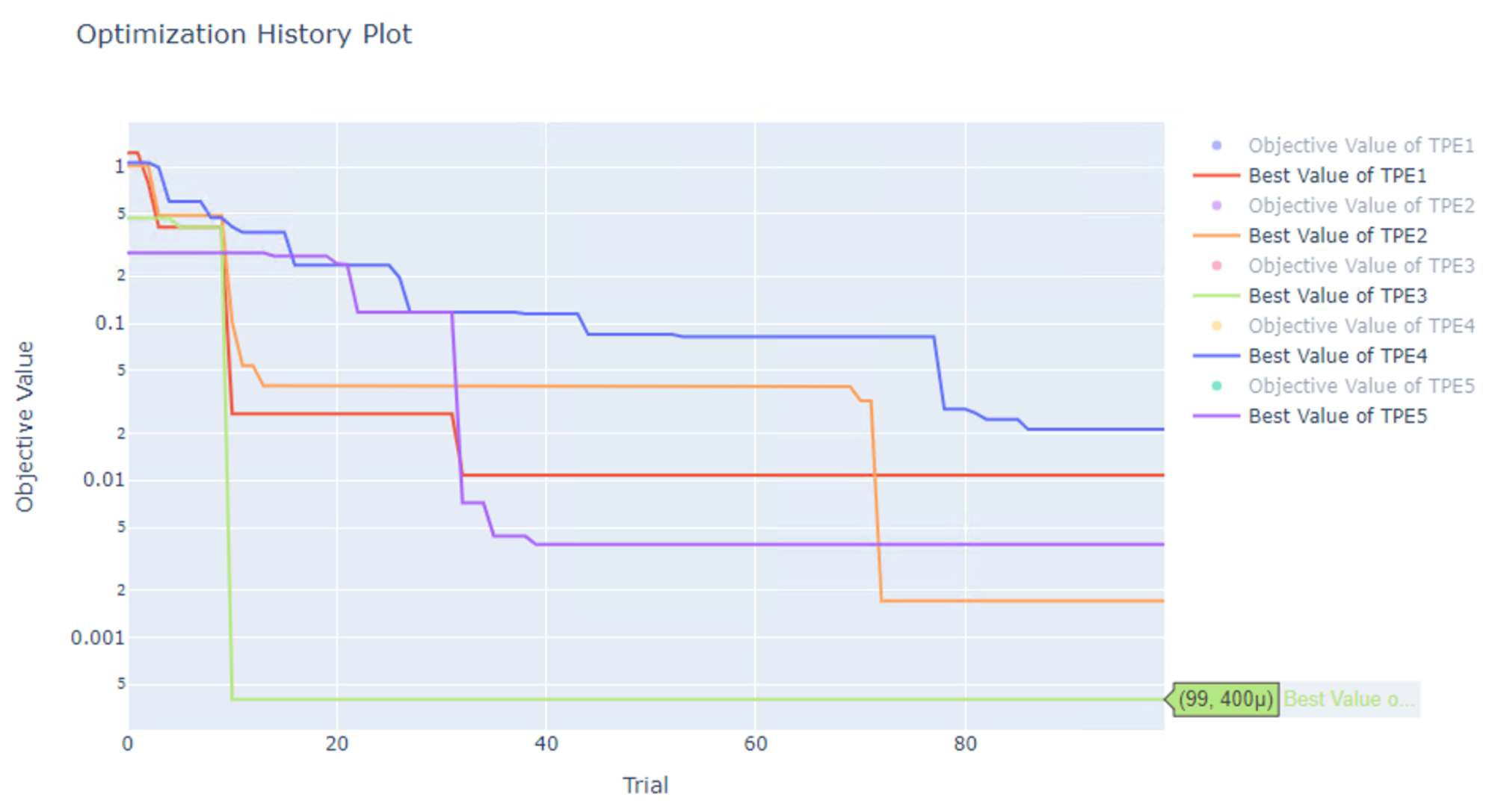
以下のグラフは最適化のヒストリーで、縦軸が目的関数の値(ここでは 2 つの NumberSlider の和)、横軸が試行回数になります。
表示されている線は各最適化で得られている最小値の変化を示したものです。
右に行くほど最適化が進むので、最小値が小さくなっていきます。
なお縦軸は対数軸になっています。
以下の表では、5回最適化を行った結果に加えて、5回中の最小値、平均値、標準偏差をあわせて記載しています。
| 1 | 2 | 3 | 4 | 5 | minimum | Average | SD | |
|---|---|---|---|---|---|---|---|---|
| TPE | 0.0108 | 0.0017 | 0.0004 | 0.0211 | 0.0039 | 0.0004 | 0.0076 | 0.0077 |
こんな人間なら一目見ただけで最小値になる変数の組み合わせ X=Y=0 がわかる簡単な問題でも、変数の組み合わせが多い(\(10^4 \times 10^4=10^8\)通り)とちゃんと0になりません。
GA を使った最適化
同様のことを Grasshopper の最適化でよく使われる GA に該当する NSGAII でも試してみます。
NSGAII のデフォルトでの設定とそれぞれの意味は以下です。
- seed : 自動計算
- 疑似乱数を生成するアルゴリズムのシード
- Mutation Probability : 自動計算
- 子集団の子個体における突然変異の確率
- 計算式 \(p_{mut} = \frac{1}{max(1, d)}\)
- d は変数の数
- 変数が 1 つの場合、突然変異の確率が 1 になりランダムになる
- 値を直接指定することも可能
- Crossover Probability : 0.90
- 子集団の生成における交叉の確率
- Crossover Method : Uniform Crossover (一様交叉)
- 子集団の生成における交叉のアルゴリズム
- Swapping Probability : 0.50
- 一様交叉において親個体のそれぞれの次元のどちらを採用するかを決定する確率
- Population Size : 50
- 各世代での個体数
結果は以下です。GA でも 0 にはなりませんでした。
| 1 | 2 | 3 | 4 | 5 | minimum | Average | SD | |
|---|---|---|---|---|---|---|---|---|
| NSGAII | 0.1799 | 0.1048 | 0.204 | 0.0445 | 0.0857 | 0.0445 | 0.1238 | 0.0595 |
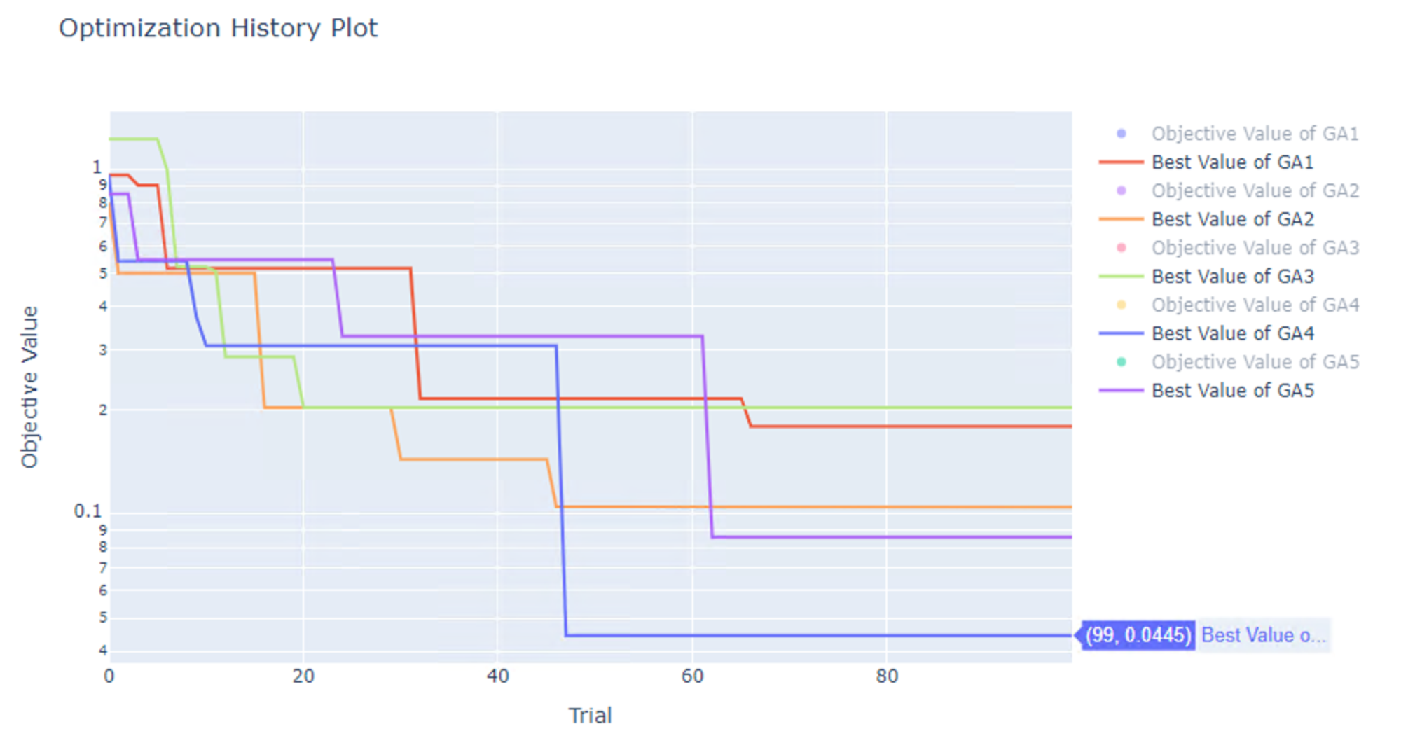
なお、 Tunny の GA のデフォルトは、1 世代 50 個体、合計 2 世代(計 100 個体)になっているため、そのままの設定で GA で最適化するにはあまり適切な設定になっていない中での結果です。
複数の手法での比較
Tunny には他の最適化手法もあるのでそれぞれやってみた結果を以下にまとめました。
| 1 | 2 | 3 | 4 | 5 | minimum | Average | SD | |
|---|---|---|---|---|---|---|---|---|
| TPE | 0.0108 | 0.0017 | 0.0004 | 0.0211 | 0.0039 | 0.0004 | 0.0076 | 0.0077 |
| NSGAII | 0.1799 | 0.1048 | 0.2040 | 0.0445 | 0.0857 | 0.0445 | 0.1238 | 0.0595 |
| Random | 0.1315 | 0.1750 | 0.1266 | 0.0974 | 0.2091 | 0.0974 | 0.1479 | 0.0394 |
| CMA-ES | 0.0000 | 0.0000 | 0.0000 | 0.0000 | 0.0000 | 0.0000 | 0.0000 | 0.0000 |
| GP-Botorch | 0.0000 | 0.0000 | 0.0000 | 0.0000 | 0.0000 | 0.0000 | 0.0000 | 0.0000 |
| GP-Optuna | 0.0000 | 0.0000 | 0.0000 | 0.0000 | 0.0000 | 0.0000 | 0.0000 | 0.0000 |
GP と CMA-ES は 100 試行でもしっかりと0になる結果が得られましたが、ほかは 0 にはなりませんでした。
TPE は 0 にはなりませんでしたが、5 回行った最適化で TPE、NSGAII、Randomの3つの中で平均値と標準偏差が小さく、4 番目に良い手法でした。
最も平均値が大きい手法はランダムで 0.1479 でしたが、NSGAII の 0.1238 と大きく変わらない結果でした。
最適化時間での比較
以上の結果を見ると 0 になっている 3 つの手法を使用すれば良いと思うかもしれません。
これらの手法の欠点は 100 試行でもかなりの時間がかかることです。
試行を 100 回行うのにかかった時間を以下にまとめています。
| sec | 1 | 2 | 3 | 4 | 5 | minimum | Average | SD |
|---|---|---|---|---|---|---|---|---|
| TPE | 3.00 | 3.04 | 3.04 | 3.11 | 3.10 | 3.00 | 3.06 | 0.04 |
| NSGAII | 2.70 | 2.77 | 2.82 | 2.82 | 2.71 | 2.70 | 2.77 | 0.05 |
| CMA-ES | 41.09 | 39.87 | 39.31 | 40.54 | 39.99 | 39.31 | 40.16 | 0.61 |
| GP-Botorch | 19.80 | 23.49 | 20.83 | 21.65 | 19.54 | 19.54 | 21.06 | 1.43 |
| GP-Optuna | 19.97 | 19.55 | 19.80 | 20.09 | 24.09 | 19.55 | 20.70 | 1.70 |
| Random | 2.32 | 2.28 | 2.31 | 2.34 | 2.32 | 2.28 | 2.32 | 0.02 |
100 試行を行う際の時間当たりに期待できる最適値を考えると真の最適解である 0 に到達はしていないですが、TPE は比較的コスパの良い手法になっていることがわかります。
注意事項
- 上記は100試行でかかる時間ですが、GP の 2 つの手法は 20 試行程度で 0 になるため、0 になる値を取得するまでの時間も実際は早いです。
- CMA-ES は一般に GP よりも早い手法ですが Tunny のデフォルトで有効になっている withMargin オプションの影響でこの例では GP よりも遅くなっています。
- 上記結果はあくまで Tunny のデフォルトの設定で最適化を行った場合の結果であって、上記の 6 つの手法のあらゆるケースでの優劣を示したわけではありません。
ではどんな設定なら結果がより良くなるか、次の章では設定をいじって確認してみます。
設定を調整して結果を改善させてみる
たくさん試行する
単純に試行回数が少なかっただけかもしれません。最適化手法の設定は変えず、100試行だったものを、10倍の1000試行でどうなるか試してみます。
対象は 100 試行では 0 にならなかった TPE、NSGAII、Random の 3 つです。
結果を以下の表にまとめています。
他のプラグインでの GA の設定は、世代数と各世代の個体数を指定します。
しかし Tunny では、各世代の個体数と総試行回数しか指定できません。
世代数は、総試行回数/個体数で決定します。
100 試行のときはデフォルトでは 1 世代 50 個体の設定のため、2世代目までしか最適化していませんでした。
今回は1000試行行うので、20世代分の計算を行っています。
結果表
| 1 | 2 | 3 | 4 | 5 | minimum | Average | SD | |
|---|---|---|---|---|---|---|---|---|
| TPE | 0.0000 | 0.0000 | 0.0000 | 0.0000 | 0.0000 | 0.0000 | 0.0000 | 0.0000 |
| NSGAII | 0.0092 | 0.0180 | 0.0041 | 0.0040 | 0.0034 | 0.0034 | 0.0077 | 0.0055 |
| Random | 0.0640 | 0.0331 | 0.0465 | 0.0174 | 0.0200 | 0.0174 | 0.0362 | 0.0173 |
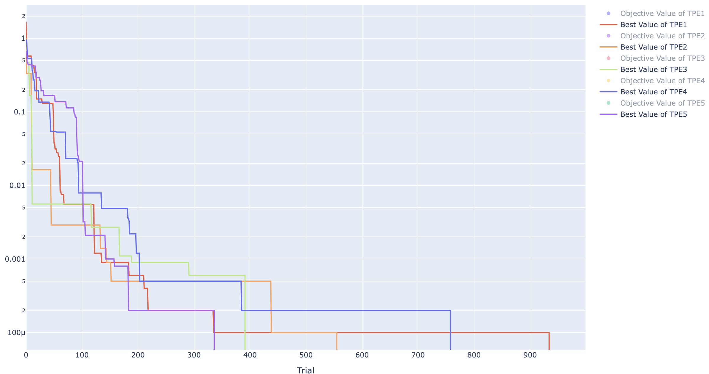
TPE ヒストリー
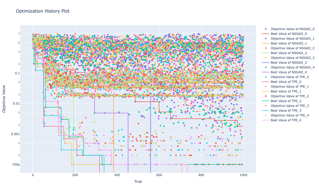
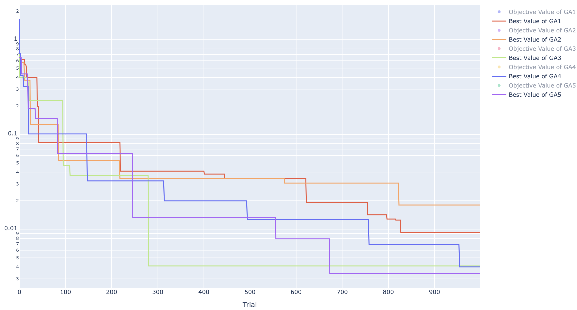
GA ヒストリー
Random ヒストリー
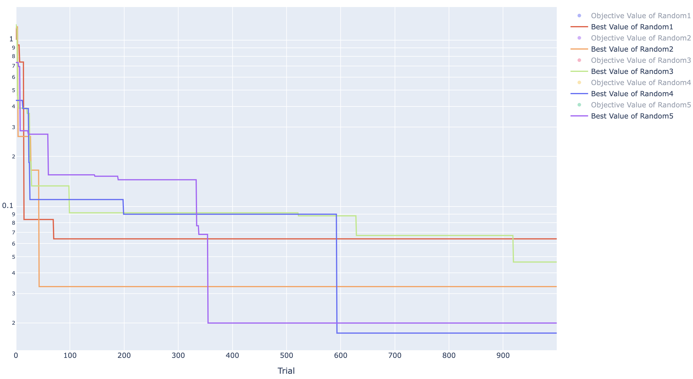
TPE はすべてのケースで 0 になりましたが GA は 0 になりませんでした。
ですが、100 試行のとき平均で 0.1238 だったのに対して、今回は 0.0077 になっており、かなり小さな値になっていることは確かです。
TPE が何試行目で 0 になったかも確認しました。
結果が以下です。
5回の平均で試行回数 596 で 0 になりました。
| trial | 1 | 2 | 3 | 4 | 5 | minimum | Average | SD |
|---|---|---|---|---|---|---|---|---|
| TPE | 935 | 556 | 392 | 759 | 337 | 337 | 595.8 | 224.4 |
単純ですが、やはり TPE も GA も試行回数を増やせばちゃんとより良い値になっていくことがわかりました。
最適化の設定を変えてみる
次に最適化手法の中での設定を変えてみます。
なお、ここでは最適化の設定の比較を行うため、内部で使用している疑似乱数のシード値を固定しています。
そのため設定の違いのみを考慮できるようにしています。
TPE 編
検討方針
TPE はデフォルトの設定でも 600 試行程度で 0 になることがわかったので、設定を変えてみてより少ない試行で 0 が得られる様になるか試してみます。
デフォルトでの設定は以下になっています。
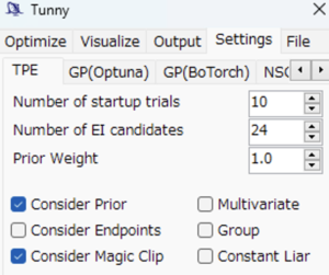
ここでは設定を変更する対象は以下の3つとします。
括弧中の値がデフォルトの値になります。
- Number of startup trials (10)
- Number of EI candidates (24)
- Consider Endpoints (False)
TPE のようなベイズ最適化に分類される手法は代理モデルを作成してそれを使用して次に探索すべき点を決定します。
代理モデルの作成には初期に行うサンプリングの数に影響を受けます。
Tunny では Number of startup trials の数字が初期のサンプリング数となり、この数だけ最適化ではなくランダムにサンプリングされます。
獲得関数を評価する際のサンプリング数が Number of EI candidates になります。
それぞれ資料[1]によると以下のように記載されています。
Number of startup trialsは総試行数の1/10程度にすると良いNumber of EI candidatesを増やすと獲得関数の評価の精度の向上が期待できる- 変数の両端を丁寧に調べたいときは
Consider Endpointsにはチェックを入れると良い
良い設定の探索
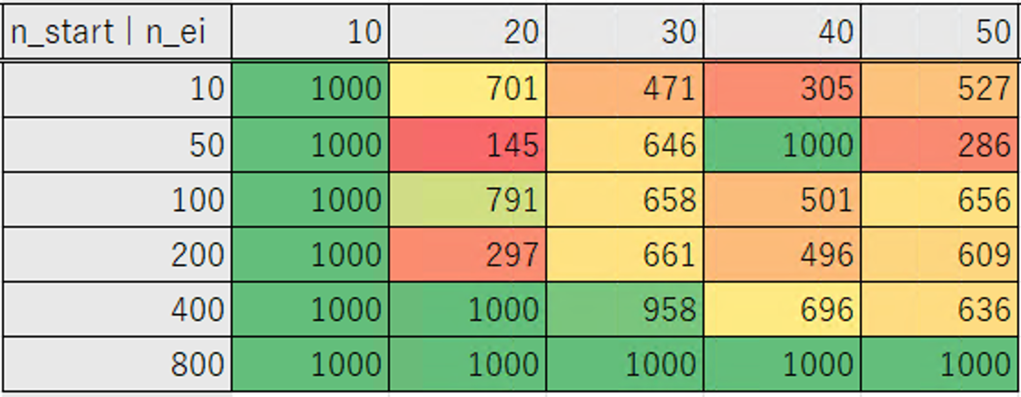
ではそれぞれを変化させて1000試行を行った際の結果です。
表は横軸が Number of EI Candidates、縦軸が Number of startup trials の数になります。
「0 が得られた試行回数」の表は 0 にならなかったケースは一律で 1000 としています。
| Consider Endpoints | 最適化結果 | 0 が得られた試行回数 |
|---|---|---|
| False | 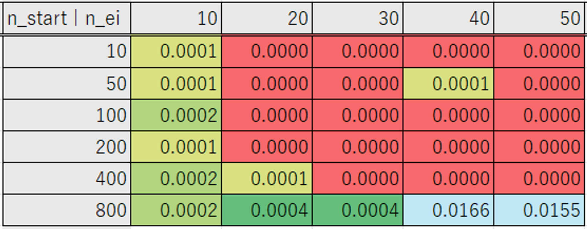 |
 |
| True | 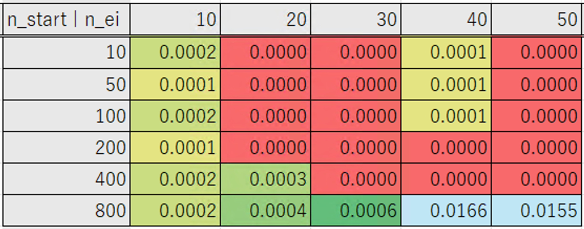 |
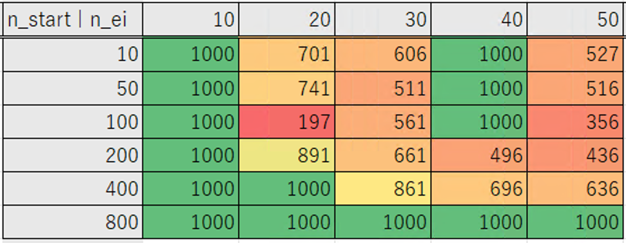 |
なおデフォルトの設定では、597 試行目で 0 の値になりました。
上記で結果が良かった以下の組み合わせで、冒頭で最適化したときのようにシード値を固定しないで5回最適化を実行したときに、結果が良くなるか確認してみます。
| case 1 | case 2 | case3 | |
|---|---|---|---|
| Number of startup trials | 50 | 50 | 100 |
| Number of EI candidates | 30 | 50 | 50 |
| Consider Endpoints | True | False | True |
Number of EI candidates が 20 のときに最も少ない試行回数で 0 になる結果が得られています。
ですが、設定によって 0 になるまでの試行回数のばらつきが大きいです。
そのため上記の設定の組み合わせの選択にあたって、ばらつきの少ない Number of EI candidates が 30 以上の結果から選択しました。
決定した設定での最適化
前節で決定した3つの設定のケースで最適化を行った結果が以下になりました。
すべて最適値は 0 になったので、0 になるまでにかかった試行回数のみをまとめています。
| 1 | 2 | 3 | 4 | 5 | minimum | Average | SD | |
|---|---|---|---|---|---|---|---|---|
| case 1 | 243 | 498 | 220 | 581 | 828 | 220 | 474 | 226 |
| case 2 | 71 | 320 | 679 | 244 | 437 | 71 | 350 | 203 |
| case 3 | 641 | 652 | 799 | 558 | 568 | 558 | 644 | 86 |
| default | 935 | 556 | 392 | 759 | 337 | 337 | 596 | 224 |
最適化のヒストリーは以下です。
対数表示のため、値が 0 になると枠外に線がでます。
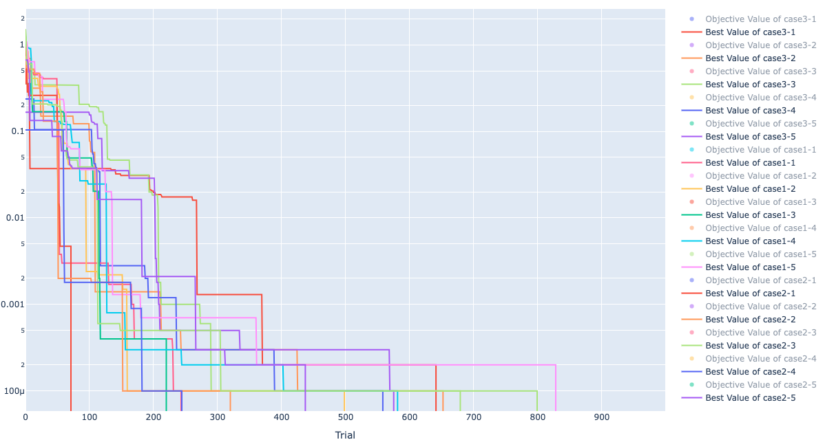
case 1, 2 はデフォルトでやった際に比べて 5 回の中の最小試行回数、平均試行回数が改善しています。
case 3 は最小試行回数、平均試行回数はデフォルトより少し悪くなっていますが、標準偏差が小さくなり、ばらつき少なく 0 の値が得られていました。
GA 編
では次に GA の設定を変更してみます。
もっとたくさんやってみる
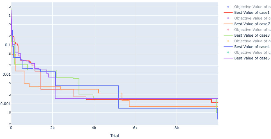
1000試行でしたが、更に10倍して10000試行でどうなるか試してみた結果が以下です。
たくさんやることにより、段々と小さくはなっていますが、0 にはなりませんでした。
| 1 | 2 | 3 | 4 | 5 | minimum | Average | SD | |
|---|---|---|---|---|---|---|---|---|
| NSGAII | 0.0011 | 0.0008 | 0.0005 | 0.0003 | 0.0015 | 0.0003 | 0.0008 | 0.0004 |
交叉方法を変える
他の手法と異なり、GA で 0 が得られないのは流石に設定が悪いと思われるので、設定を考えます。
GA では良い結果の親同士を交叉させ、より良い個体を探索していく手法なため、対象を交叉の手法にしぼり、設定を変えてみます。
Tunny では交叉の手法を以下の6つの種類から選ぶことができます。
- BLXAphaCrossover:ブレンド交叉
- SBXCrossover:疑似バイナリ交叉
- SPXCrossover:シンプレクス交叉
- UNDXCrossover:単峰正規分布交叉
- UniformCrossover:一様交叉(デフォルト設定)
- VSBXCrossover:修正疑似バイナリ交叉
デフォルトは一様交叉ですが、実数を扱うことは得意ではなく、参考文献[2]より、変数の多い最適化の場合、一様交叉は比較的性能が悪いとされています。
そのため、この手法を変更することで結果の改善が期待できます。
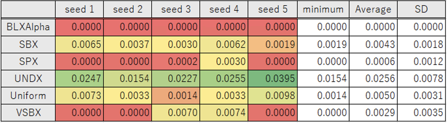
では実際に変えて最適化してみたときの結果をまとめたものが以下になります。
各手法で5回最適化を行い、それぞれで同じ条件になるように疑似乱数のシード値は同じ値にしています。
最適化結果
試行回数
Seed1 の各手法のヒストリー
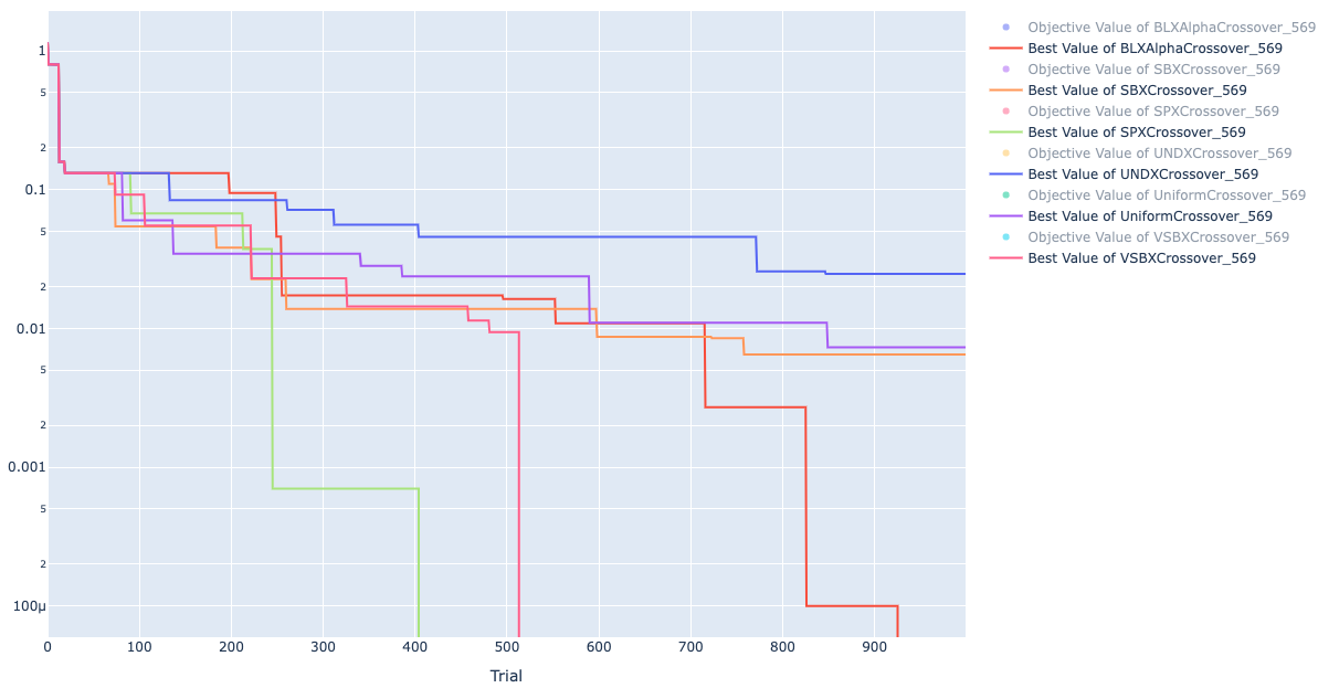
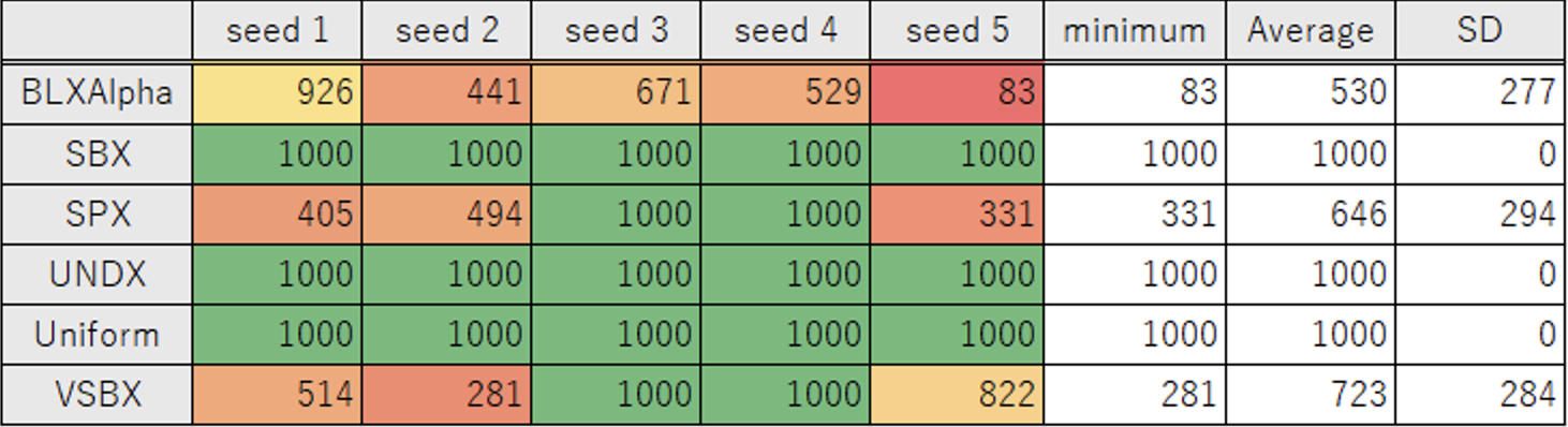
SBX, UNDX, Uniform の3つは 1 つも 0 になる結果が得られませんでしたが、BLXAlpha, SPX, VSBX は 0 を得ることができました。
特に BLXAlpha はすべてのケースかつ平均試行回数 530 で 0 が得られており、デフォルトの Uniform よりもかなり良い結果が得られました。
平均試行回数 530 は設定を調整した後の TPE での結果と同程度です。
この結果から、GA が手法として TPE に劣るというよりは、デフォルトの最適化設定が今回の最適化問題に対して適切ではなかったことがわかります。
補足
最終的に最も良かった手法である BLXAlpha(ブレンド交叉)について補足します。
ブレンド交叉は親個体の変数の組みに基づいて、その間の領域からランダムに子個体の変数の組を生成します。
子個体の変数の組は、親個体の変数の組の範囲に対して、パラメータα倍された領域の中から選択されます。
Tunny では \(\alpha = 0.5\) を使用しています。
親個体を\(P_i(x, y)\) と表すとします。
\(P_1(0, 0)\)、\(P_2(10, 5)\) とすると\(\alpha = 0.5\) のとき、この2つ親個体のブレンド交叉から作成される子個体は \(-5 \leqq x \leqq 15\)、\(-2.5 \leqq y \leqq 12.5\) の範囲で変数をとります。
まとめ
今回は Tunny を使って最適化の設定がどのように影響するかを確認していきました。
本記事で確認したのは Tunny の実装で、A+B という単純な目的関数の最適化での場合のみです。
実際の最適化問題を考えると、これ以外にも
- 多目的最適化の場合は?
- Tunny じゃなくて Wallacei や Galapagos を使った場合は?
- もっと複雑な目的関数の場合は?
- もっと変数の組み合わせが増えた場合は?
- 変数の間の相関が強い場合は?
- 制約条件を考慮した場合は?
など様々なケースが考えられ、それぞれでどのようなプラグイン、どのような設定、どのような手法、で最適化したら高速に良い結果が得られるかは変わってきます。
自分の今の設定でちゃんと必要とする精度での最適化が行われているかは常に考えながら最適化しましょう。
本記事を読んで、各設定の意味をより詳細に知りたくなった場合は、記事中の資料として参照している Tunny が最適化ライブラリとして使用している Optuna の開発者によって書かれた本[1]を一読することをおすすめします。
最適化を最適化して、よりよい最適化ライフを過ごしましょう。
参考文献
- [1] : Optuna によるブラックボックス最適化
- [2] : Stjepan Picek and Martin Golub. Comparison of a Crossover Operator in Binary-coded Genetic Algorithms. WSEAS Transactions on Computers archive, pages 1064-1073, 2010.
What Types of Optimization are Suitable
Before considering the settings, let's first examine the strengths and weaknesses of the optimization methods available in Tunny.
Tunny supports many optimization methods, so you may be unsure which one to choose. Therefore, I will first provide the strengths and weaknesses of each method as described in the official documentation, along with a flowchart for selection.
Official characteristics of each sampler (excerpt)
| RandomSampler | TPESampler | CmaEsSampler | NSGAIISampler | GPSampler | BoTorchSampler | |
|---|---|---|---|---|---|---|
| Float parameters | ✓ | ✓ | ✓ | ▴ | ✓ | ✓ |
| Integer parameters | ✓ | ✓ | ✓ | ▴ | ✓ | ▴ |
| Categorical parameters | ✓ | ✓ | ▴ | ✓ | ✓ | ▴ |
| Pruning | ✓ | ✓ | ▴ | × | ▴ | ▴ |
| Multivariate optimization | ▴ | ✓ | ✓ | ▴ | ✓ | ✓ |
| Conditional search space | ✓ | ✓ | ▴ | ▴ | ▴ | ▴ |
| Multi-objective optimization | ✓ | ✓ | × | ✓ (▴ for single-objective) | × | ✓ |
| Batch optimization | ✓ | ✓ | ✓ | ✓ | ▴ | ✓ |
| Distributed optimization | ✓ | ✓ | ✓ | ✓ | ▴ | ✓ |
| Constrained optimization | × | ✓ | × | ✓ | × | ✓ |
| Recommended budgets (#trials) | as many as one likes | 100 – 1000 | 1000 – 10000 | 100 – 10000 | – 500 | 10 – 100 |
Selection Flowchart
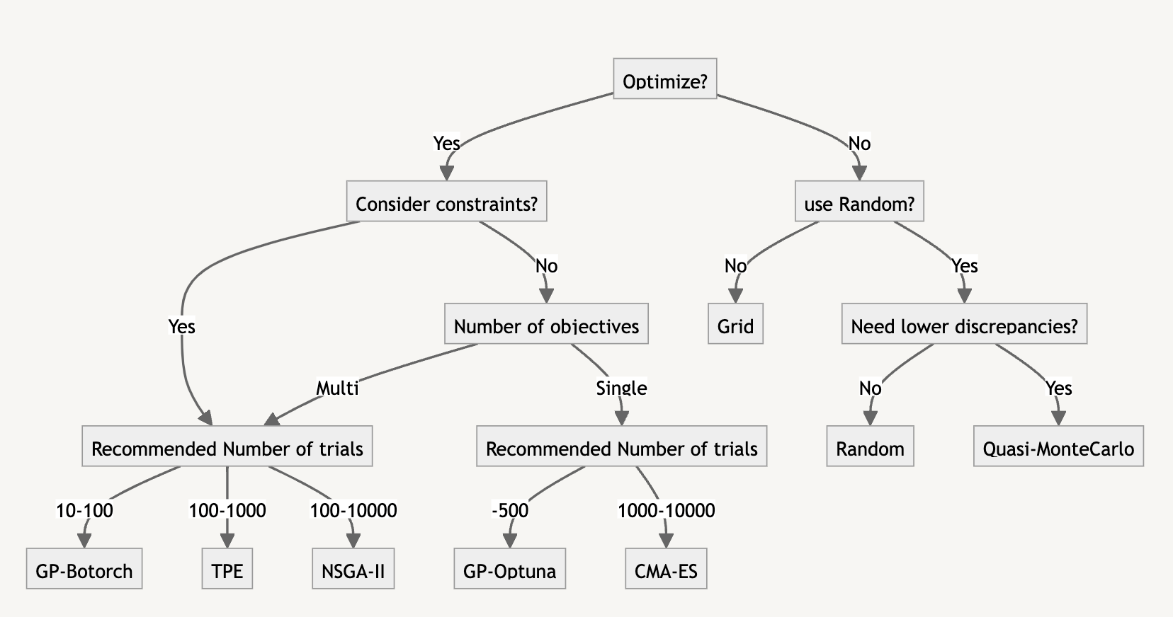
The flowchart is more of a suggestion for what to try first, but it may not necessarily be suitable for the problem you are dealing with, so it's best to experiment with various methods in practice.
Now, let's take a look at the behavior when actually using it.
Optimization with Tunny's Default Settings
Unlike other optimization plugins, Tunny's default optimization method is TPE, not GA, and it supports various methods. Since many people may not be familiar with it, let's see what happens when we run it with the default settings.
When examining optimization methods, various benchmark functions are typically used, but let's not worry about that and instead solve a simple minimization problem of the sum of two NumberSliders.
The NumberSlider takes values in the range of 0 to 1, with a precision of up to 1/10,000.
Optimization using TPE
Now, let's run the optimization using Tunny's default settings without overthinking it.
The default settings are as follows:
-
Method: TPE
-
Number of trials: 100
The optimization uses randomness in some parts, so the results change each time it is executed. Therefore, we run the optimization 5 times.
It's also possible to directly specify the seed value for generating random numbers, which allows for the reproducibility of the optimization. We will use this feature in a later chapter.
The graph below shows the optimization history, with the vertical axis representing the objective function value (in this case, the sum of the two NumberSliders) and the horizontal axis representing the number of trials.
The lines shown indicate the change in the minimum value obtained in each optimization.
As we move to the right, the optimization progresses, and the minimum value decreases.
Note that the vertical axis is on a logarithmic scale.
In the table below, in addition to the results of the 5 optimizations, we also include the minimum value, mean value, and standard deviation among the 5 runs.
| 1 | 2 | 3 | 4 | 5 | minimum | Average | SD | |
|---|---|---|---|---|---|---|---|---|
| TPE | 0.0108 | 0.0017 | 0.0004 | 0.0211 | 0.0039 | 0.0004 | 0.0076 | 0.0077 |
You're right.
Even for such a simple problem where a human can easily see at a glance that the combination of variables X=Y=0 gives the minimum value, when there are many combinations of variables (\(10^4 \times 10^4=10^8\)), it doesn't quite reach 0.
Optimization using GA
Let's try the same thing with NSGAII, which corresponds to GA, a commonly used optimization method in Grasshopper. The results are as follows. Even with GA, it didn't reach 0.
| 1 | 2 | 3 | 4 | 5 | minimum | Average | SD | |
|---|---|---|---|---|---|---|---|---|
| NSGAII | 0.1799 | 0.1048 | 0.204 | 0.0445 | 0.0857 | 0.0445 | 0.1238 | 0.0595 |
It's worth noting that Tunny's default settings for GA are 50 individuals per generation and a total of 2 generations (100 individuals in total), which are not particularly suitable for optimization using GA as is. The results shown are based on these default settings.
Comparison of Multiple Methods
Tunny offers other optimization methods as well, so I've summarized the results of trying each of them below.
| 1 | 2 | 3 | 4 | 5 | minimum | Average | SD | |
|---|---|---|---|---|---|---|---|---|
| TPE | 0.0108 | 0.0017 | 0.0004 | 0.0211 | 0.0039 | 0.0004 | 0.0076 | 0.0077 |
| NSGAII | 0.1799 | 0.1048 | 0.2040 | 0.0445 | 0.0857 | 0.0445 | 0.1238 | 0.0595 |
| Random | 0.1315 | 0.1750 | 0.1266 | 0.0974 | 0.2091 | 0.0974 | 0.1479 | 0.0394 |
| CMA-ES | 0.0000 | 0.0000 | 0.0000 | 0.0000 | 0.0000 | 0.0000 | 0.0000 | 0.0000 |
| GP-Botorch | 0.0000 | 0.0000 | 0.0000 | 0.0000 | 0.0000 | 0.0000 | 0.0000 | 0.0000 |
| GP-Optuna | 0.0000 | 0.0000 | 0.0000 | 0.0000 | 0.0000 | 0.0000 | 0.0000 | 0.0000 |
GP and CMA-ES yielded results that solidly reached 0 even with 100 trials, but the others did not reach 0.
Although TPE did not reach 0, it had the smallest mean value and standard deviation among TPE, NSGAII, and Random in the 5 optimizations performed, making it the 4th best method.
The method with the largest mean value was Random at 0.1479, but this result was not significantly different from NSGAII's 0.1238.
Comparison of Optimization Time
Looking at the above results, you might think it's best to use the 3 methods that reached 0.
The drawback of these methods is that they take a considerable amount of time, even with 100 trials.
Below is a summary of the time it took to perform 100 trials.
| sec | 1 | 2 | 3 | 4 | 5 | minimum | Average | SD |
|---|---|---|---|---|---|---|---|---|
| TPE | 3.00 | 3.04 | 3.04 | 3.11 | 3.10 | 3.00 | 3.06 | 0.04 |
| NSGAII | 2.70 | 2.77 | 2.82 | 2.82 | 2.71 | 2.70 | 2.77 | 0.05 |
| CMA-ES | 41.09 | 39.87 | 39.31 | 40.54 | 39.99 | 39.31 | 40.16 | 0.61 |
| GP-Botorch | 19.80 | 23.49 | 20.83 | 21.65 | 19.54 | 19.54 | 21.06 | 1.43 |
| GP-Optuna | 19.97 | 19.55 | 19.80 | 20.09 | 24.09 | 19.55 | 20.70 | 1.70 |
| Random | 2.32 | 2.28 | 2.31 | 2.34 | 2.32 | 2.28 | 2.32 | 0.02 |
When considering the expected optimal value per unit time for 100 trials, although TPE does not reach the true optimal solution of 0, it is evident that it is a relatively cost-effective method.
Notes
-
The 2 GP methods reach 0 in about 20 trials, so the actual time to obtain a value of 0 is faster.
-
CMA-ES is generally a faster method than GP, but in this example, it is slower than GP due to the influence of the withMargin option, which is enabled by default in Tunny.
-
The above results are based on optimization using Tunny's default settings and do not indicate the superiority or inferiority of the 6 methods in all cases.
In the next chapter, we will examine how adjusting the settings can lead to better results.
Trying to Improve Results by Adjusting Settings
Performing More Trials
It may simply be that there were not enough trials. Without changing the optimization method settings, let's see what happens when we increase the number of trials from 100 to 1000, which is 10 times more.
The targets are TPE, NSGAII, and Random, which did not reach 0 in 100 trials. The results are summarized in the table below.
Results Table
| 1 | 2 | 3 | 4 | 5 | minimum | Average | SD | |
|---|---|---|---|---|---|---|---|---|
| TPE | 0.0000 | 0.0000 | 0.0000 | 0.0000 | 0.0000 | 0.0000 | 0.0000 | 0.0000 |
| NSGAII | 0.0092 | 0.0180 | 0.0041 | 0.0040 | 0.0034 | 0.0034 | 0.0077 | 0.0055 |
| Random | 0.0640 | 0.0331 | 0.0465 | 0.0174 | 0.0200 | 0.0174 | 0.0362 | 0.0173 |
TPE history
GA history
Random history
TPE reached 0 in all cases, but GA did not reach 0.
However, compared to the average of 0.1238 with 100 trials, this time it is 0.0077, which is certainly a much smaller value.
We also checked how many trials it took for TPE to reach 0.
The results are as follows:
On average, over 5 runs, it reached 0 at 596 trials.
| trial | 1 | 2 | 3 | 4 | 5 | minimum | Average | SD |
|---|---|---|---|---|---|---|---|---|
| TPE | 935 | 556 | 392 | 759 | 337 | 337 | 595.8 | 224.4 |
It's simple, but it's clear that both TPE and GA will yield better values as the number of trials increases.
Changing Optimization Settings
Next, let's try changing the settings within the optimization methods.
Here, we fix the seed value used internally for random number generation to compare the optimization settings. This allows us to consider only the differences in settings.
TPE Section
Approach
Since TPE reaches 0 in about 600 trials even with the default settings, we will try changing the settings to see if we can obtain 0 with fewer trials.
The default settings are as follows:
Here, we will target the following three settings for modification.
The values in parentheses are the default values.
- Number of startup trials (10)
- Number of EI candidates (24)
- Consider Endpoints (False)
TPE and other methods classified as Bayesian optimization create a surrogate model and use it to determine the next point to explore.
The creation of the surrogate model is influenced by the number of initial samplings performed.
In Tunny, the Number of startup trials determines the number of initial samplings, and this many samplings are performed randomly instead of being optimized.
The Number of EI candidates is the number of samplings when evaluating the acquisition function.
According to the documentation [1], each of these is described as follows:
It is good to set Number of startup trials to about 1/10 of the total number of trials.
Increasing Number of EI candidates can be expected to improve the accuracy of the acquisition function evaluation.
When you want to carefully examine both ends of the variables, it is good to check Consider Endpoints.
Searching for Good Settings
Here are the results of performing 1000 trials while varying each setting.
The tables have Number of EI Candidates on the horizontal axis and Number of startup trials on the vertical axis.
In the "Number of trials to reach 0" table, cases where 0 was not reached are uniformly set to 1000.
| Consider Endpoints | result | Number of trials to reach 0 |
|---|---|---|
| False | |
|
| True | |
|
When using the default settings, a value of 0 was reached on the 597th trial.
Let's check if the results improve when we perform the optimization 5 times without fixing the seed value, as we did at the beginning, using the following combinations that yielded good results above.
| case 1 | case 2 | case3 | |
|---|---|---|---|
| Number of startup trials | 50 | 50 | 100 |
| Number of EI candidates | 30 | 50 | 50 |
| Consider Endpoints | True | False | True |
When Number of EI candidates is 20, the results show that 0 is reached with the fewest number of trials.
However, there is a large variation in the number of trials required to reach 0 depending on the settings.
Therefore, when selecting the above combination of settings, I chose from the results with Number of EI candidates of 30 or higher, which have less variability.
Optimization with Determined Settings
The following are the results of optimization performed using the three settings determined in the previous section.
Since the optimal value reached 0 in all cases, only the number of trials required to reach 0 is summarized.
| 1 | 2 | 3 | 4 | 5 | minimum | Average | SD | |
|---|---|---|---|---|---|---|---|---|
| case 1 | 243 | 498 | 220 | 581 | 828 | 220 | 474 | 226 |
| case 2 | 71 | 320 | 679 | 244 | 437 | 71 | 350 | 203 |
| case 3 | 641 | 652 | 799 | 558 | 568 | 558 | 644 | 86 |
| default | 935 | 556 | 392 | 759 | 337 | 337 | 596 | 224 |
The optimization history is as follows:
Due to the logarithmic display, when the value reaches 0, the line extends outside the frame.
Case 1 and 2 show improvements in the minimum and average number of trials among the 5 runs compared to the default settings.
Case 3 has a slightly worse minimum and average number of trials than the default, but the standard deviation is smaller, and a value of 0 was obtained with less variability.
GA Section
Next, let's try changing the GA settings.
Trying Even More Iterations
We tried 1000 trials, but here are the results of trying 10000 trials, which is 10 times more.
By doing many iterations, the value gradually becomes smaller, but it did not reach 0.
| 1 | 2 | 3 | 4 | 5 | minimum | Average | SD | |
|---|---|---|---|---|---|---|---|---|
| NSGAII | 0.0011 | 0.0008 | 0.0005 | 0.0003 | 0.0015 | 0.0003 | 0.0008 | 0.0004 |
Changing the Crossover Method
Unlike other methods, if GA cannot obtain 0, it is likely that the settings are poor, so let's consider the settings.
In GA, good parent individuals are crossed to explore better individuals, so we will focus on the crossover method and try changing the settings.
In Tunny, you can choose from the following 6 types of crossover methods:
- BLXApha Crossover
- SBX Crossover
- SPX Crossover
- UNDX Crossover
- Uniform Crossover ( default )
- VSBX Crossover
The default is uniform crossover, but according to reference [2], uniform crossover performs relatively poorly in optimizations with many variables.
Therefore, changing this method is expected to improve the results.
Here is a summary of the results when we actually changed the method and performed the optimization.
For each method, we performed optimization 5 times, and we set the random number seed value to the same value for each run to ensure the same conditions.
Optimization Results
Number of Trials
History of each method for Seed 1
SBX, UNDX, and Uniform did not yield any results that reached 0, but BLXAlpha, SPX, and VSBX were able to obtain 0.
In particular, BLXAlpha obtained 0 in all cases with an average number of trials of 530, which is a significantly better result than the default Uniform.
The average number of trials of 530 is comparable to the results of TPE after adjusting the settings.
From these results, we can see that GA is not inferior to TPE as a method, but rather that the default optimization settings were not appropriate for the optimization problem at hand.
Summary
In this article, we used Tunny to examine how optimization settings affect the results.
What we confirmed in this article is only the case of optimizing a simple objective function A+B using Tunny's implementation.
When considering actual optimization problems, various cases can be considered, such as:
- What about multi-objective optimization?
- What if Wallacei or Galapagos is used instead of Tunny?
- What if the objective function is more complex?
- What if the number of variable combinations increases further?
- What if constraints are taken into account?
Depending on each case, the plugin, settings, and methods that can be used to obtain good results quickly will vary.
Always consider whether optimization is being performed with the required accuracy under your current settings.
If you want to know more about the meaning of each setting after reading this article, I recommend reading the book [1] written by the developers of Optuna, the optimization library used by Tunny, which is referenced as a resource in the article.
Let's optimize optimization and lead a more optimal optimization life.
References
- [1] : Optuna によるブラックボックス最適化
- [2] : Stjepan Picek and Martin Golub. Comparison of a Crossover Operator in Binary-coded Genetic Algorithms. WSEAS Transactions on Computers archive, pages 1064-1073, 2010.
