はじめに

　皆さんの好きな双安定構造は何ですか？日常生活で様々な双安定構造を利用している皆さんにとって，お気に入りを一つ選ぶのは難しいかもしれません。今回の記事では，私の推し双安定構造について紹介します。

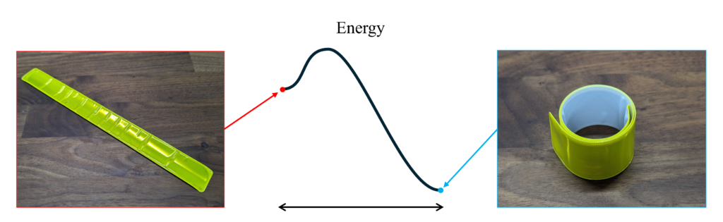
　双安定構造とは，2つの異なる安定状態（双安定性）を示す構造です。以前の記事で，ヒンジキャップを例に挙げて双安定構造について紹介しました。双安定構造は，弾性エネルギーが極小となるときに安定状態となり，エネルギーの山を乗り越えることでもう一方の安定状態に遷移することにも触れました。

スラップバンド

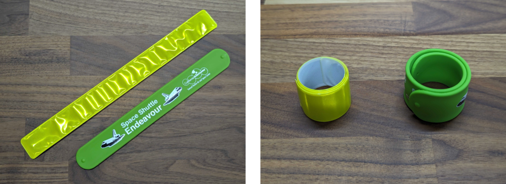
　私の推し双安定構造は，スラップバンドです。 スナップブレスレットやワンタッチバンドなどとも呼ばれます[1]。夜間に遠くから視認可能な反射材として（もしくは双安定性を楽しむための玩具として）使用する方も多いと思います。

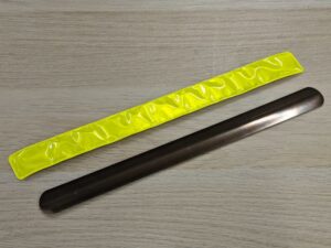
　スラップバンドは腕などに打ち付けると巻き付いて簡単に装着できます。これは伸ばした状態でも丸めた状態でも安定する双安定性によって実現できる挙動です。打ち付けた際に弾性エネルギーの山を乗り越え，伸ばした状態で蓄えられていた弾性エネルギーが解放されて，瞬時にもう一方の安定状態（丸まった状態）に遷移します。 　スラップバンドのカバーを外して中身を確認すると，双安定性を実現する一枚の薄い鋼板が入っています。以降は，この板自体をスラップバンドと呼ぶことにし，その特徴について解説していきます。

曲面形状

　スラップバンドが他の双安定構造と比べて特徴的である理由は，その曲面形状にあります。スラップバンドの曲面形状は，伸縮や切断なく平面に展開することが可能です。

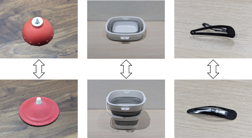
　これに対して，曲面を利用した双安定構造の多くは，3次元空間で平面に展開するには，伸縮や切断，折曲げを必要とする曲面形状となっています。次の写真に例を示します。

\scriptsize{
非可展面（※1）を利用した双安定構造の例。\\
（左）バウンシングボール（※2）という複曲面（半球面）の玩具。\\
　　　裏返した状態で地面に落とすと，蓄えた弾性エネルギーを解放して高く跳ね上がる。\\
（中）折畳み可能なバケツ。100円ショップで550円で購入した。\\
　　　灰色のゴム部が裏返った状態で安定するため，容積を小さくして収納可能。\\
（右）ヘアピン。平板を端部で接続することで複曲面形状を作っている（※3）。}

このような曲面は，曲げ剛性による復元力と面内剛性による復元力の釣り合いによって双安定性を生み出しています。（変形の際に面内にも伸縮するため，人の手で大きく変形させるにはゴムのような軟質材を用いるか，金属でもヘアピンのように寸法を小さくする必要があります。）

　上述したように，スラップバンドは平面に展開可能な曲面形状となっています。このような曲面は曲げ変形の際に面内に伸縮しないため，曲面を作っただけでは双安定構造にはなりません。では，どのように双安定性を生み出しているのでしょうか？

\tiny{
※1　図学の曲面分類では可展面は単曲面と平面であり切断や折曲げを許容する[2]。ここでは\text{globally developable}でない曲面として「非可展面」と記述した。
\\
※2　\text{Bowl}派と\text{Ball}派がいる。\text{Hip Hop Bouce Fidget Toy}という呼称もある。\\
※3　連続的でないので厳密には曲面の定義から外れているが，巨視的に見ると複曲面ということで容赦いただきたい。}

残留応力

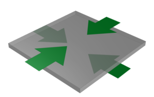
　スラップバンドが双安定性を有するカギは，残留応力にあります。スラップバンドを平面にすると，表と裏で直交する方向に残留応力が発生しています。 これにより，それぞれの方向には曲がった状態で安定するような復元力が働きます。しかし，平面に展開可能な曲面（単曲面）が同時に双方向に曲率を持つ（すなわち複曲面になる）には，面が伸縮する必要があります。そのため，スラップバンドはどちらか一方にのみ曲率を持つ形（単曲面）で変形します。

　一方向に曲率を持った際に，もう一方に対しては断面二次モーメントが大きくなることで残留応力のみでは曲がらずに安定します。これがいずれの方向にも成立することで双安定性が生まれています。

作ってみる

　原理を理解しやすいように，身近な材料を用いて工作してみましょう。

■ 用意するもの

• 輪ゴム
• ハサミ
• 曲げに対して適度な復元力を持つ平板 \small{〇\>硬めのクリアファイルや厚紙が良いと思います。今回は名刺を使用しました。} \small{〇\>できるだけ均質で等方性の材料の方が，意図した変形になりやすいです。} \small{〇\>できるだけクリープ（応力緩和）しない材料の方が，長期的に使用できます。}

■ 手順

1. 用意した平板の角にスリットを入れます。
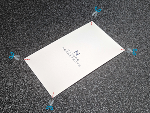
2. 図のように輪ゴムを挿入します。輪ゴムの張力を調整し均等にします。張力が足りない場合は輪ゴムを複数本付けると良いでしょう。
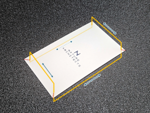
3. 完成！

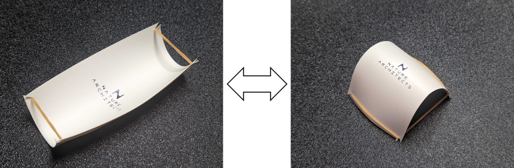
上の工作では残留応力による復元力を輪ゴムを使って表現していますが，今回取り上げたスラップバンドでは，塑性加工により生じた残留応力を利用しています。コンベックスメジャーを塑性変形するまで曲げることで，双安定性を持つスラップバンドを作製した動画もあります[3]。

また，CFRP（炭素繊維強化樹脂）を用いることで，成形時の熱収縮異方性によって表裏で直交する残留応力が発生するように積層構成を工夫するだけで，同様の双安定性を生み出すこともできます[4-6]。（具体的には，積層構成を[0_n/90_n]などの非対称クロスプライにします。）

類似構造

　スラップバンドの双安定性メカニズムは，他の構造にも活用されています。今回は，類似のメカニズムが利用されている双安定構造を2つ紹介します。

ハエトリグサ

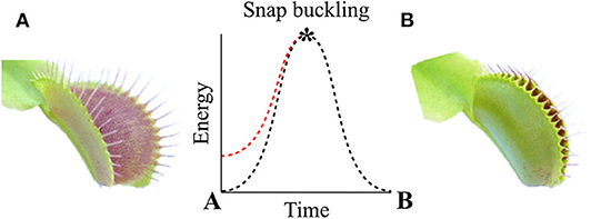
　ハエトリグサはスラップバンドと同じ双安定機構を利用していると言われています[7-9]。二枚貝のような葉の内側に生えた感覚毛が刺激されると，細胞が収縮して葉を閉じます。このとき，開いた状態で蓄えられた弾性エネルギーを利用することで，葉を素早く閉じて獲物を捕食することができます。 \scriptsize{[7]より引用}

双安定STEM

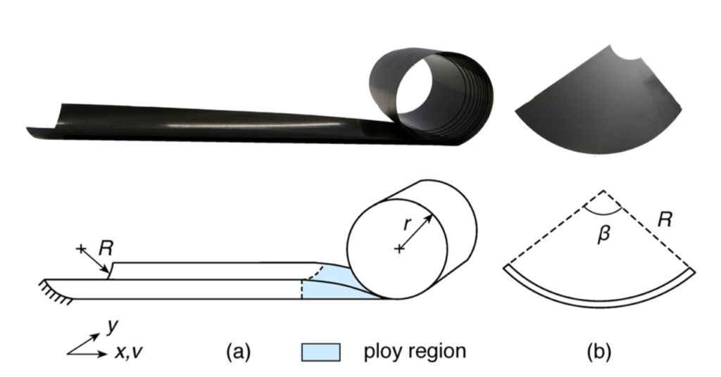
　宇宙展開構造物の構成要素に利用される伸展ブームに，STEM(Storable Tubular Extendible Member)という種類があります[10]。輸送時は省スペース化のためコイル状に巻き付けた状態で収納し，宇宙で伸展させて使用します。 \scriptsize{[11]より引用}

STEMの中でも，巻き取り状態と伸展状態の両方を安定して保持できる双安定性を持つものがあります[11,12]。このようなSTEMはCFRPで製造されます。双安定STEMは巻き取り状態で反力を押さえつける構造が不要なため，収納機構を簡略化できます。また，一部が変形した際に伸展状態に移行する自己伸展性を持たせることも可能です（巻き取り状態に移行しやすいスラップバンドとは逆ですね）。このような収納性や自己伸展性を活用して，地上でもアンテナや三脚に用いられることもあります[13,14]。

　また，スラップバンドでは2つの安定状態において凸面が反転しますが，双安定STEMの場合は形状が変化しても凸面が同じ側にあります。これは，単に残留応力だけがメカニズムではなく，CFRPの特性を利用することで実現されています。このメカニズムについては，後で詳しく見ていきます。

双安定性の条件

　スラップバンドがどのような条件で双安定性が成立するのか気になると思うので，数式を用いて説明します。（高校物理の範囲を逸脱しながらも，簡単な連続体力学の数式のみで挙動を記述できるのもスラップバンドの推しポイントです）

　残留応力を有する単曲面に対して，安定状態となるひずみエネルギーの極小点が複数存在する条件を導出します。

エネルギー算出

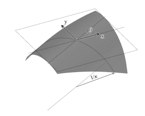
　一様曲率の単曲面が面内変形が生じずに変形するとき，曲率\kappaとその方向\thetaの２つで曲面状態を記述できます。図のように，角度\theta\>(0\le\theta< \pi)方向を軸とした曲率\kappaを有するとき，xy座標での曲率は次のように表されます。（ひずみ変換行列を利用して導出しています）

[\kappa]=
\begin{bmatrix}
c^2 & s^2 & sc\\
s^2 & c^2 & -cs\\
-2sc & 2sc & c^2-s^2\\
\end{bmatrix}
\begin{bmatrix}
0\\ \kappa\\ 0\\
\end{bmatrix}
=\kappa \begin{bmatrix}
\sin^2\theta\\ \cos^2\theta\\ 2\sin\theta\cos\theta\\
\end{bmatrix}
=\kappa/2 \begin{bmatrix}
1-\cos2\theta\\ 1+\cos2\theta\\ 2\sin2\theta\\
\end{bmatrix} \tag{1}

ここで，初期状態での曲率半径R( > 0)とし，残留応力によりモーメント荷重m_0が発生しているものとします。曲率はy方向にあり，モーメント荷重はx方向に作用しているとします。

[\kappa_0]=
\begin{bmatrix}
0\\ 1/R\\ 0\\
\end{bmatrix},
[m_0]=
\begin{bmatrix}
m_0\\ 0\\ 0\\
\end{bmatrix}\tag{2}

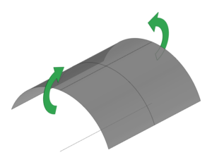
このとき，初期状態から曲率変化[\Delta\kappa]および単位寸法あたりに発生するモーメント荷重[m]は次のようになります。

[\Delta\kappa]=[\kappa]-[\kappa_0]=\kappa/2
\begin{bmatrix}
1-\cos2\theta\\ 1+\cos2\theta\\ 2\sin2\theta\\
\end{bmatrix}-\begin{bmatrix}
0\\ 1/R\\ 0\\
\end{bmatrix}\\\tag{3}

[m]=[D][\Delta\kappa]+[m_0]\tag{4}

ここで，[D]は平面応力状態における曲げ剛性行列であり，等方性材料の場合は次のように表されます。

[D]=D\begin{bmatrix}
1 & \nu & 0 \\
\nu & 1 & 0\\
0 & 0 & (1-\nu)/2\\
\end{bmatrix}\tag{5}

係数Dは板厚tの平板に対して中央中立面を仮定したとき，D=\frac{t^3E}{12(1-\nu^2)}となります。（板厚方向に積分したときのモーメントのつり合いから導出されます。詳細を知りたい方は以前の記事で述べた古典積層理論をご参照ください。）

式(4)より，単位面積あたりのひずみエネルギーUは次のようになります。

\begin{align}
U &= 1/2[\Delta\kappa]^T[D][\Delta\kappa]+[\Delta\kappa]^T[m_0]\\
 &= \frac{1}{2} \left\{
 \frac{D}{R^2}-\kappa(D\kappa+m_0)-
\kappa\left\{\frac{D(1+\nu)}{R}+\left(\frac{D(1-\nu)}{R}+m_0\right)\cos2\theta\right\}
\right\} \tag{6}
\end{align}

極値判定

ひずみエネルギーUが\kappaと\thetaに対して停留点（極値もしくは鞍点）であるためには，各変数に関する微分が0である必要があります。また，その点でヘッセ行列が正定値ならば，極小であると言えます。

\frac{\partial U}{\partial\theta}=\frac{\partial U}{\partial\kappa}=0, \>|H_U(\theta,\kappa)|>0\Rightarrow \text{Local minimum}

\thetaに注目すると，\theta=0,\pi/2のときに\frac{\partial U}{\partial\theta}=0となります。

(A)\theta=0のとき，

初期状態\kappa=1/Rで\frac{\partial U}{\partial\kappa}=0となります。この点において，ヘッセ行列は次のようになります。

H=\begin{bmatrix}
D &  0 \\
0 & \frac{2}{R}(\frac{D(1-\nu)}{R}+m_0)\\
\end{bmatrix}\tag{7}

これにより，

\begin{align}
detH=\frac{2D}{R}\left(\frac{D(1-\nu)}{R}+m_0\right) > 0\\
m_0 > -\frac{D(1-\nu)}{R}\tag{8}
\end{align}

のとき，この点は極小となります。

(B) \theta=\pi/2のとき，

\kappaによる偏微分は

\frac{\partial U}{\partial\kappa}=m_0+D\kappa-D\nu/R \tag{9}

となり，\kappa = \frac{\nu}{R}-\frac{m_0}{D}で\frac{\partial U}{\partial\kappa}=0となります。この点において，ヘッセ行列は次のようになります。

H=\begin{bmatrix}
D &  0 \\
0 & 2(\frac{\nu}{R}-\frac{m_0}{D})(-\frac{D(1-\nu)}{R}-m_0)\\
\end{bmatrix}\tag{10}

これにより，

\begin{align}
detH=2\left(\frac{D\nu}{R}-m_0\right)\left(-\frac{D(1-\nu)}{R}-m_0\right)>0\\
m_0<-\frac{D(1-\nu)}{R}, \frac{D\nu}{R}< m_0\tag{11}
\end{align}

のとき，この点は極小となります。

　式(8)と式(11)より，\frac{D\nu}{R}< m_0のとき，次の2点において安定状態となることが分かります。

　A. \theta=0, \kappa = \frac{1}{R}

　B. \theta=\pi/2, \kappa = \frac{\nu}{R}-\frac{m_0}{D}\> (< 0)

このとき，Bでの曲率は負となり凸面が反転することが分かります。

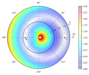
例として，D=1, \nu=0.3, R=1, m_0=0.5のときのひずみエネルギーを可視化します。グラフでは，径方向に\kappa\> (-1.5＜\kappa＜1.5)，周方向に2\theta\> (0\le\theta<\pi)としています。 グラフを見てもAとBにおいて極小となっていることが分かります。また，スラップバンドにおいて丸めた状態をA，伸ばした状態をBとしたとき，次の様子も表現できています。

• B（伸ばした状態）におけるエネルギーはA（丸めた状態）よりも高く，Aに遷移する範囲が大きい
• B（伸ばした状態）における曲率はA（丸めた状態）よりも0に近く，平面に近い状態となっている。

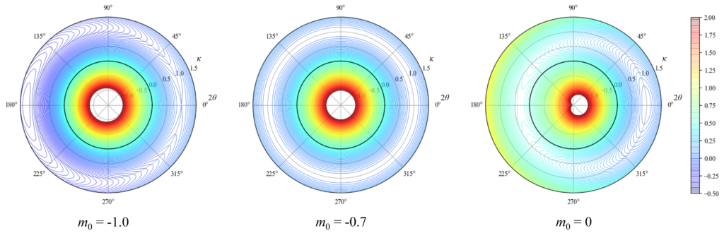
また，m_0が上記双安定条件でないときのひずみエネルギーの様子を下図に示します。これらの場合，極小が１つ，もしくは存在しないことが分かります。（m_0=-\frac{D(1-\nu)}{R}とすると，図中央のように常に\frac{\partial U}{\partial\theta}=0となり角度変化による剛性が0となる[15]ことも面白いですね。）

双安定STEMでは

上記では，曲面が双安定構造となるとき，2つの安定状態において必ず凸面が反転しました。一方で，類似構造として紹介した双安定STEMでは凸面が同じ面となります。これは，FRPの異方性を利用することで成立する挙動です。 直交異方性材料の曲げ剛性行列は次のように記述できます。

[D]= \frac{t^3}{12}
\begin{bmatrix}
\frac{E_X}{1-\nu_{XY}\nu_{YX}} & \frac{\nu_{YX}E_Y}{1-\nu_{XY}\nu_{YX}} & 0\\
\frac{\nu_{YX}E_Y}{1-\nu_{XY}\nu_{YX}} & \frac{E_Y}{1-\nu_{XY}\nu_{YX}} & 0\\
0 & 0 & G_{XY}\\
\end{bmatrix}
=
\begin{bmatrix}
D_{11} & D_{12} & 0\\
D_{12} & D_{22} & 0\\
0 & 0 & D_{66}\\
\end{bmatrix} \tag{12}

これを用いて，上の等方性材と同じように初期状態での曲率半径R(> 0)，モーメント荷重m_0としたときのエネルギーについて考えます。

U=1/2[\Delta\kappa]^T[D][\Delta\kappa]+[\Delta\kappa]^T[m_0]

\thetaに注目すると，\theta=0,\pi/2のときに\frac{\partial U}{\partial\theta}=0となります。

(A) \theta=0のとき

等方性材のときと同様，\kappa=1/Rで\frac{\partial U}{\partial\kappa}=0となります。この点において，ヘッセ行列は次のようになります。

H=\begin{bmatrix}
D_{22} &  0 \\
0 & \frac{2}{R}(\frac{2D_{66}}{R}+m_0)\\
\end{bmatrix} \tag{13}

絶対値が正のとき，この点は極小となります。

\begin{align}
detH=\frac{2D_{22}}{R}\left(\frac{2D_{66}}{R}+m_0\right) > 0\\
m_0 > -\frac{2D_{66}}{R} \tag{14}
\end{align}

(B) \theta=\pi/2のとき，

\frac{\partial U}{\partial\kappa}=m_0+D_{11}\kappa-D_{12}/R \tag{15}

であり，\kappa = \frac{D_{12}}{D_{11}R}-\frac{m_0}{D_{11}}のときに\frac{\partial U}{\partial\kappa}=0（臨界点）となります。

この点において，ヘッセ行列は

H=\begin{bmatrix}
D_{11} &  0 \\
0 & \frac{2}{D_{11}^2R^2}(D_{12}-m_0R)\{-D_{11}D_{22}+(D_{12}+2D_{66})(D_{12}-m_0R)\}\\
\end{bmatrix}\tag{16}

となり，その絶対値が正であるとき極小となります。

\begin{align}
detH= \frac{2}{D_{11}R^2}(D_{12}-m_0R)\{-D_{11}D_{22}+(D_{12}+2D_{66})(D_{12}-m_0R)\}>0\\
m_0<\frac{1}{R}(D_{12}-\frac{D_{11}D_{22}}{D_{12}+2D_{66}}),\frac{D_{12}}{R} < m_0 \tag{17}
\end{align}

式(14)と式(17)より，(\alpha) \frac{D_{12}}{R} < m，もしくは(\beta) -\frac{2D_{66}}{R} < m < \frac{1}{R}(D_{12}-\frac{D_{11}D_{22}}{D_{12}+2D_{66}})のとき，次の2点で安定状態となります。

　A. \theta=0, \kappa = \frac{1}{R}

　B. \theta=\pi/2, \kappa = \frac{D_{12}}{D_{11}R}-\frac{m_0}{D_{11}}

(\alpha)のときは，等方性材のときと同様にBにおいて\kappa < 0となり凸面が反転します。

一方で(\beta)のときは，Bにおいて\kappa> 0となり凸面が同じ方向になります。このとき，次が成立する必要があります。

\begin{align}
-\frac{2D_{66}}{R} < \frac{1}{R}(D_{12}-\frac{D_{11}D_{22}}{D_{12}+2D_{66}})\\
D_{11}D_{22} < (D_{12}+2D_{66})^2  \tag{18}
\end{align}

また，-\frac{2D_{66}}{R} < 0より，

\begin{align}
0 < D_{12}-\frac{D_{11}D_{22}}{D_{12}+2D_{66}}\\
D_{11}D_{22} < D_{12}(D_{12}+2D_{66}) \tag{19}
\end{align}

であればm_0=0，すなわち残留応力によるモーメント荷重が無い状態でも双安定となります。

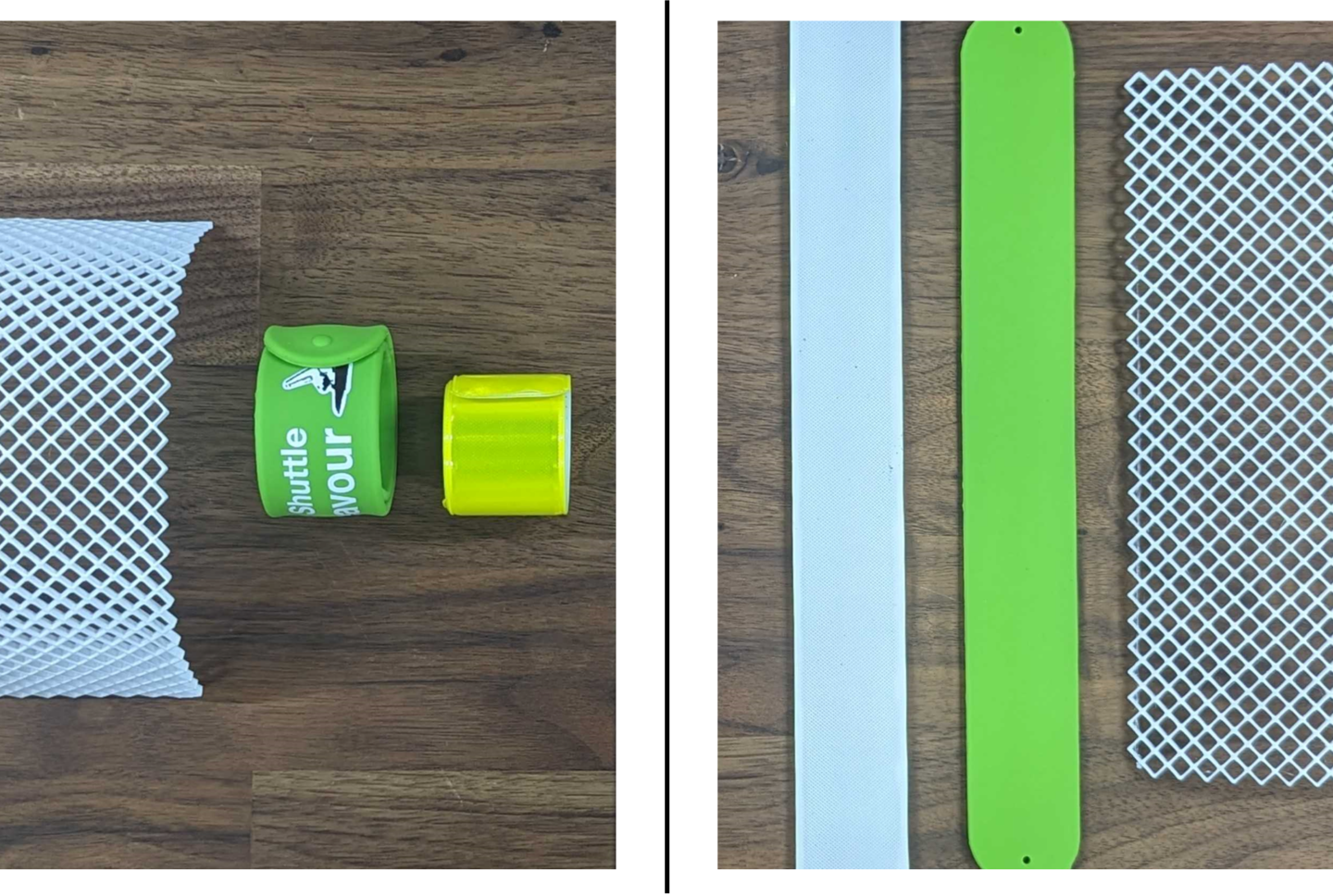
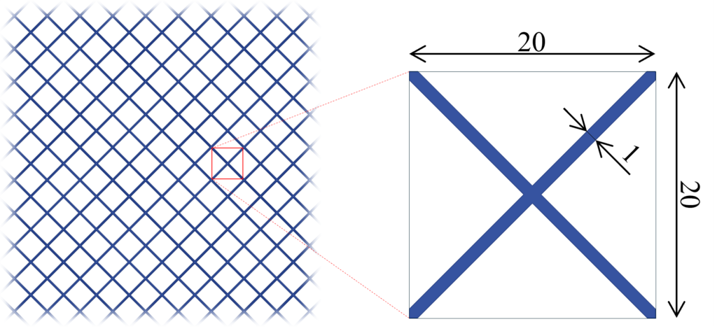
ここで，式(12)に示した直交異方性材の剛性行列を見ると，ポアソン比やせん断剛性が大きければ式(18)や式(19)条件を満たすことが分かります。そのようなメタマテリアルとして，例えば次のような格子状の構造を考えます。 ポアソン比が0.3の均質等方性材料を用いて上記形状を作成したとき，有限要素法を用いて計算すると，面内剛性マトリクスは次のようになりました。

[A]= \begin{bmatrix}
\frac{E_X}{1-\nu_{XY}\nu_{YX}} & \frac{\nu_{YX}E_Y}{1-\nu_{XY}\nu_{YX}} & 0\\
\frac{\nu_{YX}E_Y}{1-\nu_{XY}\nu_{YX}} & \frac{E_Y}{1-\nu_{XY}\nu_{YX}} & 0\\
0 & 0 & G_{XY}\end{bmatrix}
= \begin{bmatrix}
E & 0.96E & 0\\
0.96E & E & 0\\
0 & 0 & 0.88E \end{bmatrix}

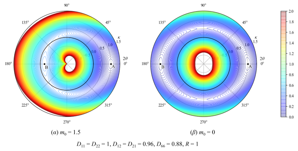
この構造を用いた場合，(α)m_0=1.5, (β)m_0=0としたときのひずみエネルギーをグラフにすると次のようになります。 右のグラフのように，異方性材料を用いることで，凸面の反転なく双安定構造を作ることができます。 今回はメタマテリアルの観点から格子構造を用いましたが，実際の双安定STEMにおいては，長手方向に対して±45度方向に繊維が配向されたCFRPを用いることで同様に双安定性が成立しています。

　直感的な解釈としては，±45度方向に湾曲した状態を保とうすることで双安定が成立していると理解することもできます。

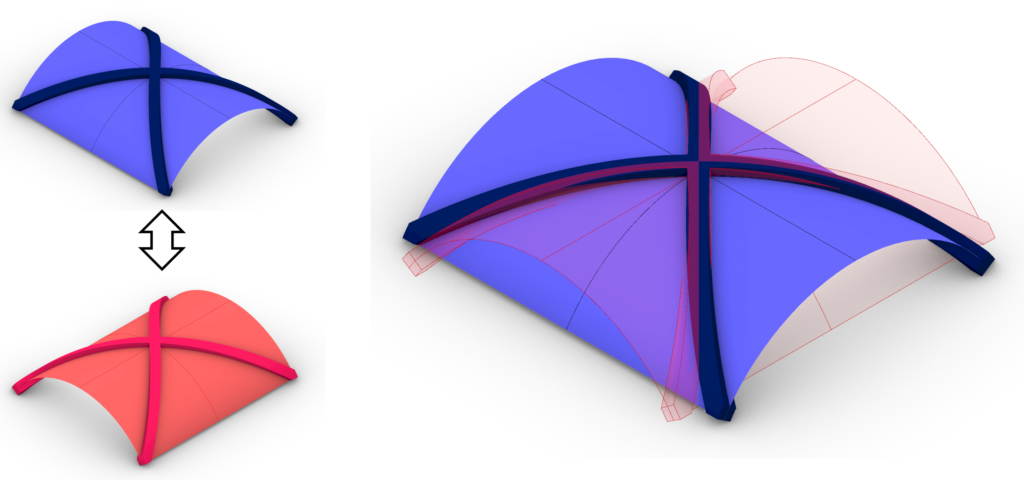
　以上のように，スラップバンドの双安定性が成立する条件を考えることで，その特徴について理解することができました。

• 等方性材料を用いた場合は，２つの安定状態で必ず凸面が反転する。
• 直交異方性材料を用いることで，凸面を反転させることなく双安定性を成立させることも可能である。そのとき，残留応力は不要な場合もある。

おわりに

　ここまでお読みいただきありがとうございました。スラップバンドやSTEMの双安定性について，工作や数式を交えて解説していきました。少しでも構造の面白さが伝われば幸いです。皆さんも好きな双安定構造について深堀りしてみてください。

参考文献

[1] Wikipedia. Slap bracelet.（参照2024年5月）

[2] 舘知宏. 複曲面／ねじれ面／単曲面. 図学研究 第51巻. 2017年7月

[3] youtube.com. Make SNAP BANDS from Unusual Materials. （参照2024年5月）

[4] Michael W. Hyer. Calculation of the room-temperature shapes of unsymmetric laminates. 1981.

[5] Michael W. Hyer. Some Observations on the Cured Shape of Thin Unsymmetric Laminates. Journal of Composite Materials. 1981, 15(2).

[6] Min Sun et al. A Unified High-Order Semianalytical Model and Numerical Simulation for Bistable Polymer Composite Structures. Polymers 2022, 14(4), 818

[7] Esser et al. Artificial Venus Flytraps: A Research Review and Outlook on Their Importance for Novel Bioinspired Materials Systems. Frontiers in Robotics and AI. 2020, 7(25).

[8] Dario Lunni et al. Plant‐Inspired Soft Bistable Structures Based on Hygroscopic Electrospun Nanofibers. Asvanced Materials Interfaces. 2020, 7, 1901310

[9] Anna S. Westermeier et al. How the carnivorous waterwheel plant (Aldrovanda vesiculosa) snaps. Proceedings of the royal society B. 2018, 285(1878).

[10] 宇宙科学研究所, 超軽量展開宇宙構造物 （参照2024年5月）

[11] Alex Brinkmeyer et al. Effects of Long-Term Stowage on the Deployment of Bistable Tape Springs. Journal of Applied Mechanics. 2016, Vol.83

[12] 秋人渡邊. 双安定性ブーム. JP6590218B2. 2016

[13] https://revolve-tec.com/ （参照2024年5月）

[14] https://www.rolatube.com/ （参照2024年5月）

[15] SIMON D. GUEST et al, Journal of Mechanics of Materials and Structures. 2021, 6, 1-4

[16] Evripides G Loukaides. Expanding the Build Plate: Functional Morphing 3D Printed Structures Through Anisotropy. Frontiers in Materials. 2020, 7, 159.