
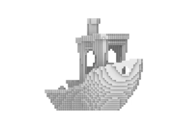
発想 idea
弊社は、日々「カタチ」について探求をしている会社です。すでに世の中にあるカタチを理解しながら、まだ世にないカタチをどうやって生み出すかについても研究を続けています。そんな新たな形を創造する方法として、計算機を用いた形状生成について調査している過程で、marching cubesという手法に出会いました。
marching cubes[1]は、1987年にLorensenとClineによって発表されたコンピュータグラフィックスアルゴリズムであり、3次元の離散スカラー場から等値面の多角形メッシュを抽出します。このアルゴリズムは、主にCTやMRIスキャンデータ画像などの医療用ビジュアライゼーションに用いられます。
また、marching cubesは、3Dに使用することを意図して作られたアルゴリズムですが、このアルゴリズムを2Dに適用することも可能であり、その場合はmarching squaresと呼ばれています。
marching squaresの代表的な使用例は、天気図での等圧線の描画や地図上の等高線の描画です。地図上で格子状にマッピングされた離散的な情報をもとに、大気圧の滑らかな変化を推測し、地図に重ねて表示します。marching squaresは計算が軽量であることから、時々刻々変化する気圧の測定値を瞬時に変換し、観測する人間にとって感覚的に理解しやすい画像を届けることが可能となっています。
marching squaresはすでに幅広く利用されている技術ですが、今回はあえてこのmarching squaresをRhinocerossのGrasshopper上で1から処理を実装することでアルゴリズムを理解しながら、色々な画像を処理、生成して遊んでみたいと思います。
調査 research
まずは、marching squares法のアルゴリズムの理解から始めます。
Wikipedia[2]に大変分かりやすい説明があったので、補足を加えながら引用させていただきます。
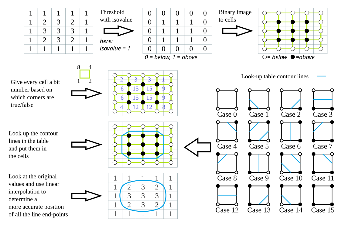
アルゴリズムの手順
①データの二値化
2Dスカラー場の値を、基準値(しきい値)を使用して二値化し、白黒のピクセル画像にします。
- 基準値以上の場合は「1」とする。
- 基準値未満の場合は「0」とする。
②輪郭セルの作成
二値化された画像の2x2のブロックに対して、1つの「輪郭セル」を構成します。この輪郭セルのグリッドは、元の2Dスカラー場に比べて各方向に1セル小さくなります。(下の図では、もともと5*5の離散スカラー場を持っていましたが、この処理により4*4のグリッドに変わります。)【ここから各セルごとの処理します】
③セルインデックスの決定
輪郭セルの4つの角(バイナリ値1または0を保持)を時計回りに巡りながらセルインデックスを作成します。このインデックスは4ビットの値となり、0から15までの16通りの状態のどれかを表します。④ルックアップテーブルの参照
生成されたインデックスを使用して、事前に用意されたルックアップテーブルを参照します。ルックアップテーブルには、セル内のどの辺に輪郭線が通るべきかが指定されています。marching squareで使用するのは、このルックアップテーブルに記載された基本16種の形状だけです。⑤線形補間
セルの辺上で、元の2Dスカラー場の値を使用して、輪郭線の正確な位置を線形補間によって補正します。これにより、先ほどの基本16種を変形しより滑らかな境界線を得ることができます。
①②を実行後、③~⑤をセルごとに順々に処理することで等値線を表す境界線が描かれていきます。
16種の形状パターンを4bitのバイナリに対応させて処理する過程が、萌えポイントですね。
構築 build
marching squares法のアルゴリズムの手順で確認した、16種の基本形状を用いて境界線を表現する④の状態と、線形補間を適用した⑤の状態には少し開きがあるので、marching squaresの実行段階を以下の3つの状態に分けて考えます。
| state | name | description |
|---|---|---|
| 1 | marching squares threshold | しきい値によって2値化した状態。ドット絵の状態。 |
| 2 | marching squares 16 pattern | セルインデックスに対応した16種の基本形状を割り当てた状態。グリッドに対して45度の境界線を持つことができ、表現力が向上。 |
| 3 | marching squares linear interpolation | しきい値に分解する前のスカラー場の値を使って線形補間を適用した状態。滑らかな境界線を表現可能。 |
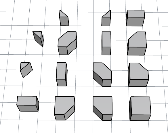
16種の基本形状
16種の基本形状をrhino上で、立体のソリッドポリサーフェスとしてモデリングしました。2Dの画像処理を想定しているので、高さは仮置きで1として統一しています。下の図を見ると15種しかないように見えますが、「左上の何もない空間」も形状を表す状態の1つとしてカウントしているので、全16種になります。
state 2の処理では、この16個のブロックを積み木のように配置していくことで、形状を再現します。
バイナリ演算
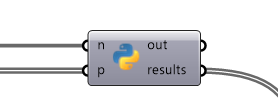
grasshopper上でのバイナリ演算は、Python Scriptコンポーネントの中で、pythonコードとして処理しました。セルの周囲4点のノードのバイナリ値(0か1)を並べて、4bitの数値として読み取り、それを10進数の0~15の数字として出力します。この0~15の数字に対応したブロックを、先ほどの形状群から選択し、そのセルの位置に配置すればmarching squaresを適用した形状が作られていきます。
Python 3 Script
# n: 正方形ピクセル画像の縦横ピクセル数
# p: 各ノードの値(0or1)(ex n=64のときpは1024個のリストデータ)

def convert_to_matrix(n, p):
    matrix = []
    for i in range(n):
        row = p[i*n:(i+1)*n]
        matrix.append(row)
    return matrix

def calculate_p_values_as_int(n, p):
    # 一次元リストを二次元行列に変換
    p_matrix = convert_to_matrix(n, p)

    results = []
    for i in range(n-1):
        for j in range(n-1):
            # 4ビットのバイナリ数値を文字列として取得
            binary_str = f"{p_matrix[i][j]}{p_matrix[i][j+1]}{p_matrix[i+1][j+1]}{p_matrix[i+1][j]}"
            # バイナリ文字列を整数に変換
            int_value = int(binary_str, 2)
            results.append(int_value)
    return results

#各輪郭セルのバイナリ値(0~15)
results = calculate_p_values_as_int(n, p)
print(results)
線形補間
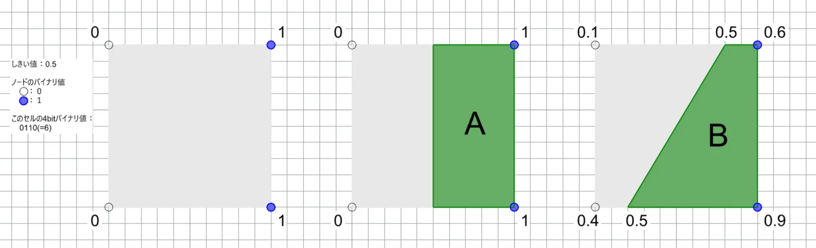
アルゴリズムの⑤にある線形補間を施すことで出力される画像をより滑らかにすることができます。線形補間の例として、あるセル(4bitバイナリ値「0110」)に対する処理を下図に表しました。
まず、一番左の図形は、スカラー場に対して、各ノードの値をしきい値0.5によって、01のバイナリ値に変換した状態です。このセルについて、左上から時計回りにノードのバイナリ値を読み取ると「0110」となっています。「0110」は10進数で読み取ると「6」のブロックに対応しているため、そのブロックを配置します。画像中央のAの形状がそれを表しており、アルゴリズムの実行段階としては、state 2になります。
このAの形状を得た後に、0と1の中間にある角について、しきい値で分類する前のスカラー値(ここでは、0.1, 0.6, 0.9, 0.4)を用いて、線形補間によりしきい値(0.5)の座標を推測し、形状を変形させる操作を行います。これによって、得られたBの形状が、アルゴリズムの実行段階としては、state 3になります。
実行 test
上記で構築した要素を組み合わせて、Marching squares法の実行環境をGrasshopper上に作成しました。
以下にそれを使用した実施例として、①ピクセル画像の境界を滑らかに変換した例と、②ランダム生成したスカラー場の等高線可視化した例を紹介します。
① ピクセル画像の境界を滑らかに変換
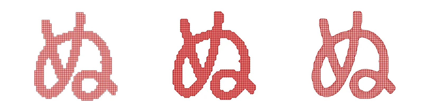
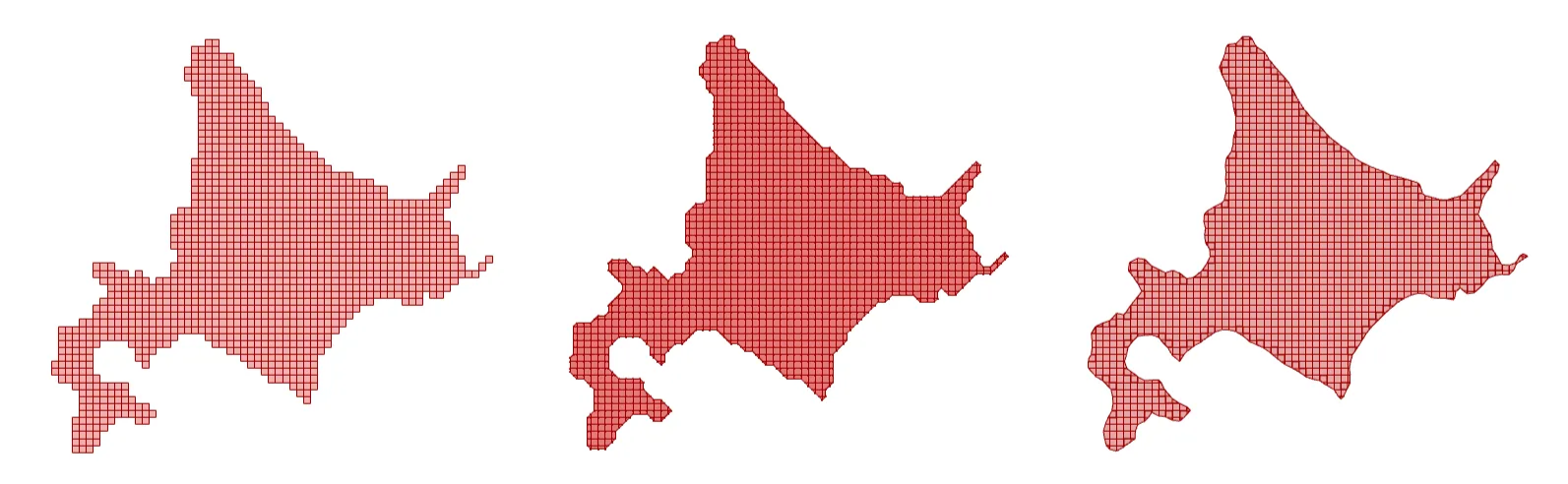
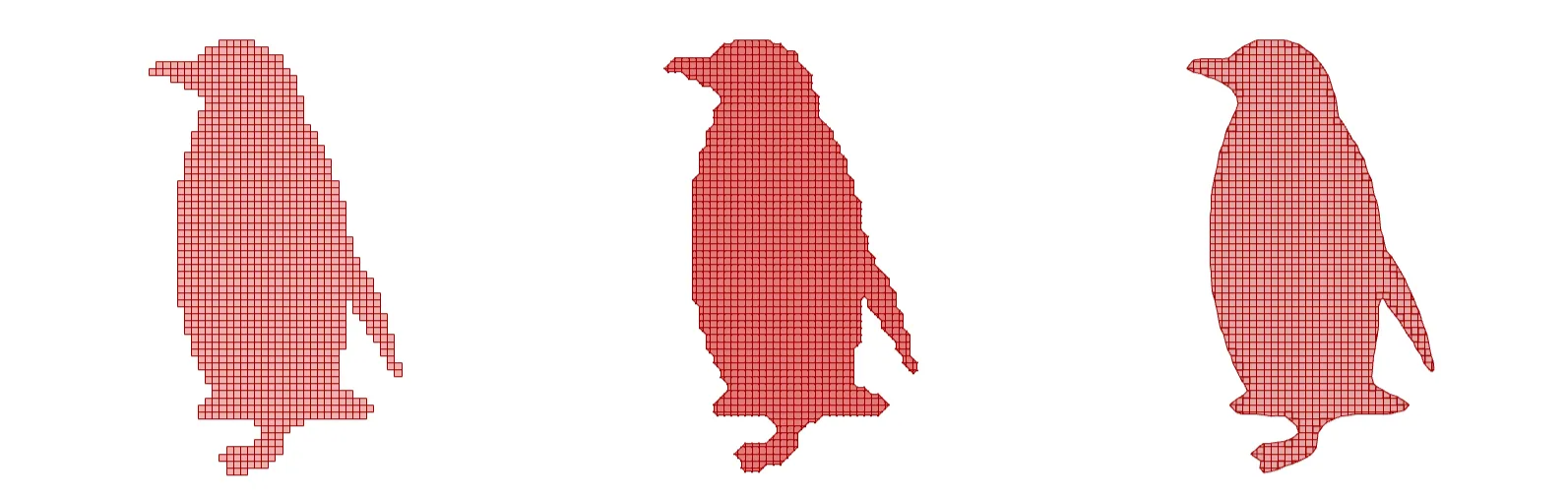
ここでは、様々な64×64のピクセル画像に対して、marching squaresを適用した過程を、3つの実行段階ごとに示します。左からstate1, state2, state3の順で並べてあります。
どの画像も右に行くほど境界滑らかで、綺麗な画像に見えると思います。一番左のドット絵では、1つのセルサイズよりも細い形状は表現しきれませんが、一番右の画像では細い部分もちゃんと表現できています(北海道の根室半島がきれいに表現できています)。また、車の丸いタイヤ形状やペンギンなどの曲線形状では、ピクセル表現では不自然に感じる場合がありますが、marching squaresを適用することで自然な滑らかさを感じることができるようになります。

グレースケール画像との比較
上記の画像処理では、state 2からstate 3に変換する際に、元画像の情報として、各ノードに与えられた0~1の間の数値を持ったスカラー値を使用しています。このスカラー値を光度に対応させて描画したグレースケール画像と、そこからmarching squaresを適用して境界を抽出した結果を比較してみましょう。
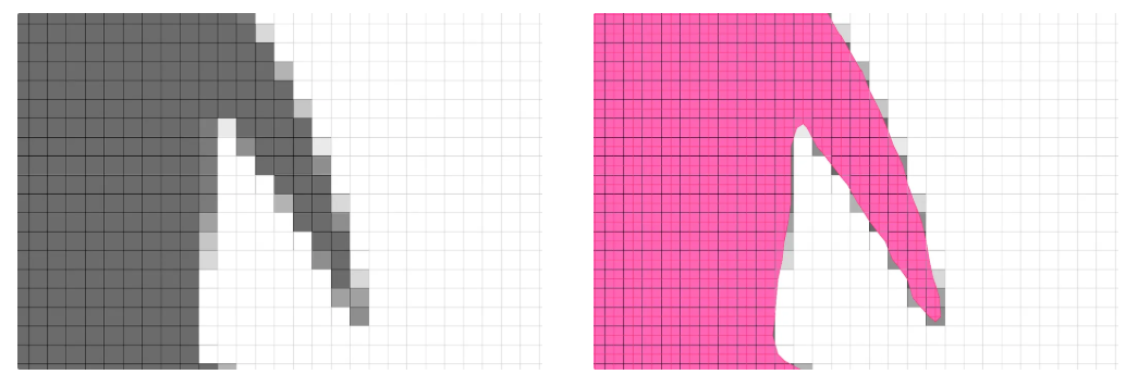
下図は、ペンギンのひれの部分の拡大図です。左側のグレースケール画像の場合は、ピクセルの直角な境界が目立ち、自然なひれの形状には見えません。一方で、右側に重ねたのmarching squaresによる画像は、同じ情報量でありながら、滑らかな形状が人の目でも観測しやすくなっています。
② ランダム生成したスカラー場の等高線可視化
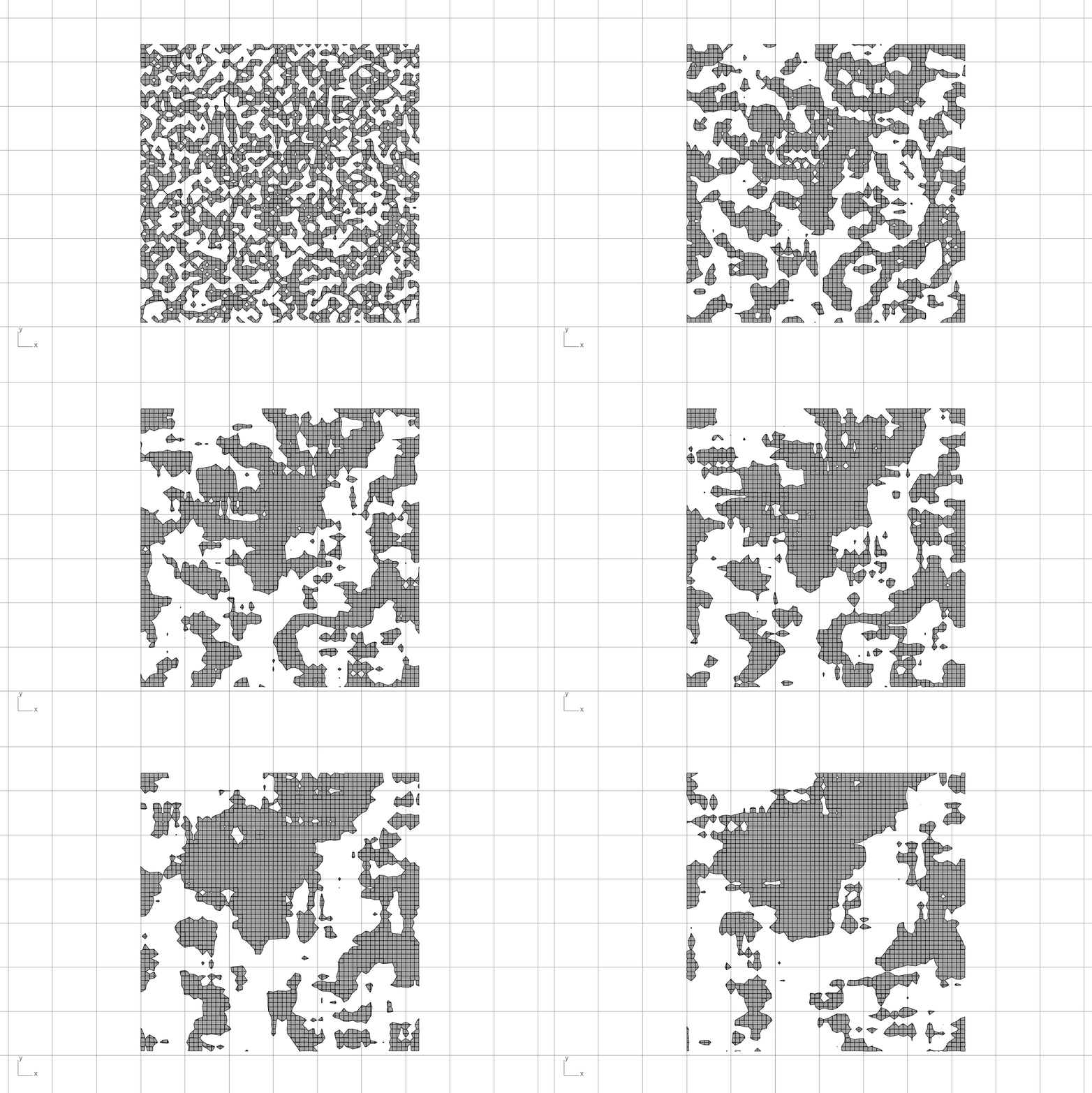
続いて、64×64のグリッドにランダムな数値を与えてスカラー場を構築し、そのスカラー場に対してmarching squaresを実行した例を示します。スカラー場には、平均化のフィルタをかけており、フィルタを徐々に強くしていくことでランダム値の変化を平坦にしていった様子をgifにしてみました。
もっとも細かい模様から始まって、徐々に大きな塊の模様に変化していきます。この画像自体に物理的な意味はありませんが、スカラー場に意味を持たせれば有用な形状を生成することも期待できます。
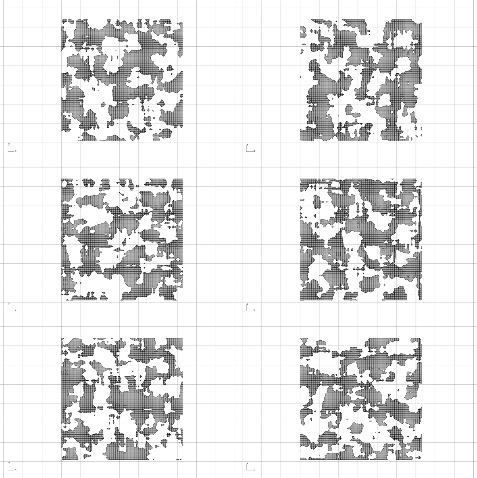
つぎに、一定の平均化フィルタを用いて、元のランダム値のシード値を振った場合の画像をgif化してみました。こうすると、同程度の形状粒度を持った、様々な画像が得られます。
私には存在しない大陸をかたどった無数の地図を生成しているように見えますが、皆さんは何を創造するでしょうか。
おまけ extra
冒頭でmarching squaresは、marching cubesの2Dバージョンであるという説明をさせていただきました。ここでは少しだけ、marching cubesにトライした結果をまとめておきます。
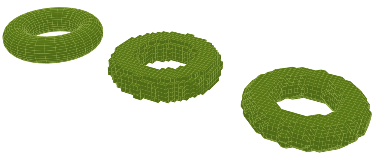
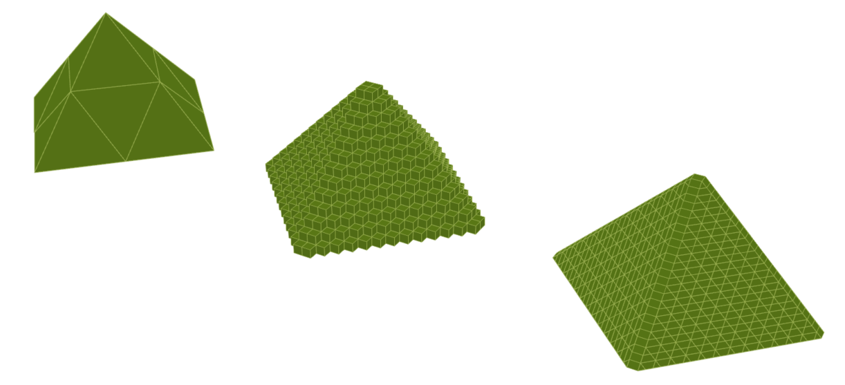
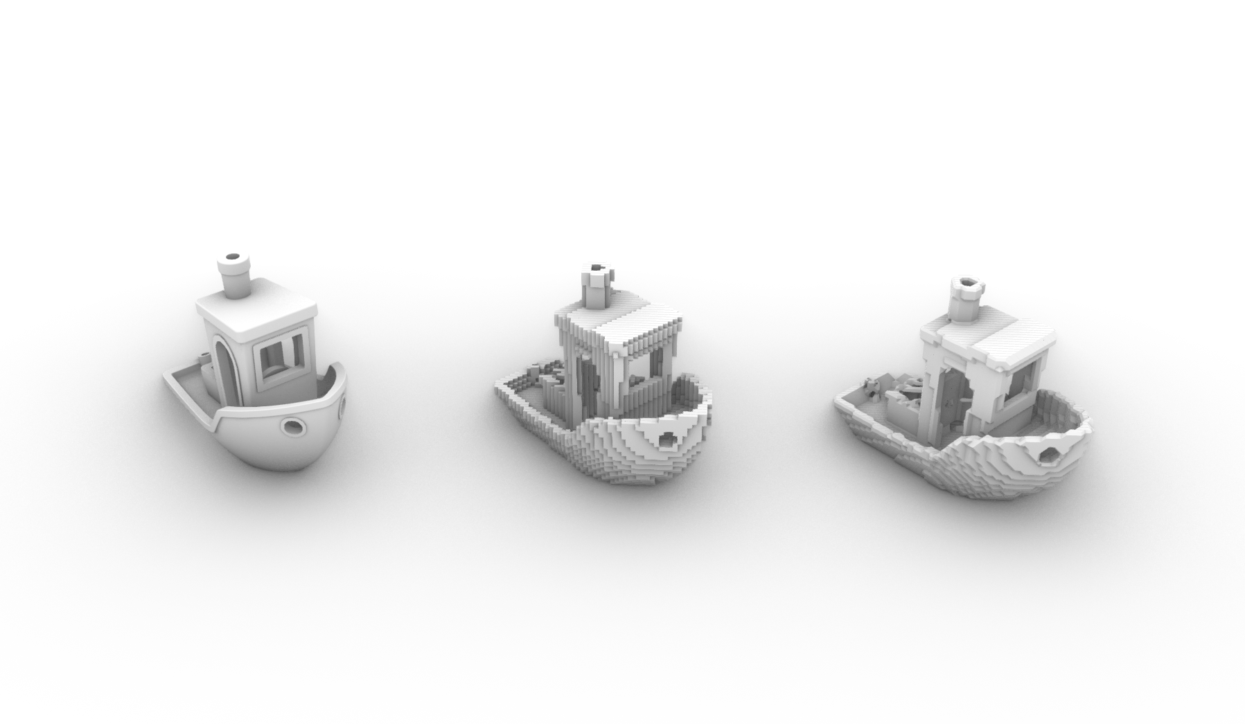
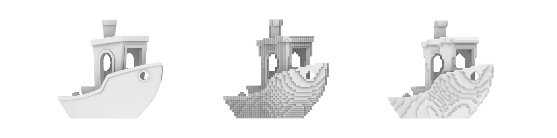
marching cubesでは、marching squaresの1つのセルが、立方格子に拡張され8つの頂点を持ちます。この点の0, 1によって表現される基本形状は、下図の30個の図形をXYZ軸に回転させて重複を除いた256個の形状です。これは、8つの頂点のバイナリ値によって作られる8bitのバイナリ値が表現できる0~255の全256通りに等しい数になります。
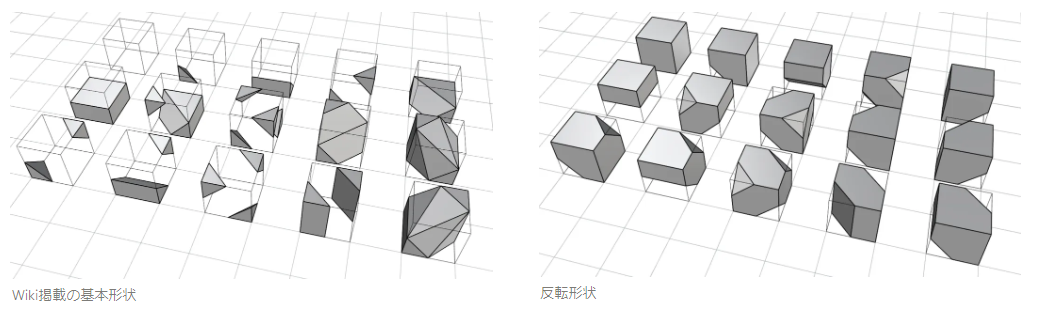
下にいくつかの形状について、表現したい正解データと、立方体のみで表現したボクセル表現と、maching cubesのstate2に相当する256個の基本形状ブロックで表現した状態を並べてみました。
3次元形状になると256通りのブロックを用いても、なかなか滑らかと言える表現力を持たせることができませんでした。3次現空間においても、2次元と同じく線形補間が可能ですが、grasshopperでの実装はそれなりに複雑になりそうなので、今回は取り組みではstete 2までとしましたが、marching cubesの効果の片鱗は感じられたかと思います。
振り返り review
今回は、marching squares法を用いて、ピクセル画像から滑らかな境界線を作成したり、ランダムに生成したスカラー場から新たな境界線を作成したりしてみました。marching squaresの手法自体は、グレースケール画像を加工して境界を見やすくしているだけとも言えますが、出力された滑らかな形状を人が見ることで、その感じ方、印象は大きく変わるため、そこから得られる情報、発想に差が出てくるかと思います。
使用したソフト
[1] Rhino 8, Grasshopper
参考文献、サイト
[1] https://dl.acm.org/doi/10.1145/37402.37422
[2] https://en.wikipedia.org/wiki/Marching_squares
[3] https://www.youtube.com/watch?v=0ZONMNUKTfU&ab_channel=TheCodingTrain
[4] https://jamie-wong.com/2016/07/06/metaballs-and-webgl/
[5] https://ragingnexus.com/creative-code-lab/experiments/algorithms-marching-squares/
[6] https://www.3dbenchy.com/
idea
We are a company that is constantly exploring "shapes". While understanding shapes that already exist in the world, we continue to research how to create shapes that do not yet exist. In the process of investigating computer-based shape generation as a way to create such new shapes, we came across a method called marching cubes.
Marching cubes[1] is a computer graphics algorithm announced by Lorensen and Cline in 1987 that extracts a polygonal mesh of isosurfaces from a three-dimensional discrete scalar field. This algorithm is mainly used for medical visualization such as CT and MRI scan data images.
Although marching cubes is an algorithm intended to be used in 3D, it can also be applied to 2D, in which case it is called marching squares.
A typical example of the use of marching squares is drawing isobars on weather maps and contour lines on maps. Based on discrete information mapped in a grid on a map, it estimates smooth changes in atmospheric pressure and displays them overlaid on the map. Marching squares is a lightweight technology that can instantly convert ever-changing atmospheric pressure measurements and deliver images that are easy for observers to understand.
Marching squares is already a widely used technology, but this time I will implement the process from scratch on Grasshopper in Rhinoceross to understand the algorithm and play around with processing and generating various images.
Research
First, let's start by understanding the algorithm of the marching squares method.
There was a very easy-to-understand explanation on Wikipedia [2], so I will quote it with some additional information.
Steps of the algorithm
① Data binarization
The 2D scalar field values are binarized using a reference value (threshold) to create a black and white pixel image.
- If it is equal to or greater than the reference value, it is set to "1".
- If it is less than the reference value, it is set to "0".
② Creating a contour cell
For each 2x2 block of the binarized image, one "contour cell" is created. This contour cell grid is one cell smaller in each direction than the original 2D scalar field. (In the image below, we originally had a 55 discrete scalar field, but this process changes it to a 44 grid.)【From here, we process each cell individually】
③ Determining the cell index
Create a cell index by going around the four corners of the contour cell (which hold binary values 1 or 0) in a clockwise direction. This index is a 4-bit value that represents one of 16 possible states from 0 to 15.④ Referencing the lookup table
The generated index is used to refer to a lookup table prepared in advance. The lookup table specifies which side of the cell the contour line should pass through. Only the 16 basic shapes listed in this lookup table are used in marching square.⑤ Linear Interpolation
On the edge of the cell, the exact position of the contour is corrected by linear interpolation using the original 2D scalar field value. This allows you to deform the 16 basic types and obtain a smoother boundary line.
After executing ① and ②, ③ to ⑤ are processed in order for each cell to draw the boundary line representing the isoline.
The process of processing the 16 shape patterns by making them correspond to 4-bit binary is the cute part.
Build
There is a slight difference between state ④, which expresses the boundary line using 16 basic shapes, and state ⑤, which has linear interpolation applied, as confirmed in the procedure of the marching squares algorithm, so we will divide the execution stage of marching squares into the following three states.
| state | name | description |
|---|---|---|
| 1 | marching squares threshold | The state binarized by threshold. The pixel art state. |
| 2 | marching squares 16 pattern | The state in which 16 basic shapes corresponding to the cell index are assigned. It is possible to have a 45-degree boundary line relative to the grid, improving expressiveness. |
| 3 | marching squares linear interpolation | Linear interpolation is applied using the value of the scalar field before it is decomposed into a threshold value. Smooth boundary lines can be expressed. |
16 basic shapes
16 basic shapes were modeled as solid polysurfaces on rhino. Since 2D image processing is assumed, the height is temporarily set to 1. Looking at the diagram below, it looks like there are only 15 types, but the "empty space in the upper left" is also counted as one of the states that represent the shape, so there are a total of 16 types.
In state 2 processing, the shape is reproduced by arranging these 16 blocks like building blocks.
Binary operations
Binary operations on Grasshopper were processed as python code in the Python Script component. The binary values (0 or 1) of the four nodes around the cell are lined up, read as a 4-bit number, and output as a decimal number from 0 to 15. Select the block corresponding to this number from the group of shapes mentioned earlier and place it at the cell position to create a shape with marching squares applied.
Python 3 Script
# n: Number of pixels in the width and height of a square pixel image
# p: Value of each node (0 or 1) (ex. when n=64, p is 1024 list data)

def convert_to_matrix(n, p):
matrix = []
for i in range(n):
row = p[i*n:(i+1)*n]
matrix.append(row)
return matrix

def calculate_p_values_as_int(n, p):
# Convert one-dimensional list to two-dimensional matrix
p_matrix = convert_to_matrix(n, p)

results = []
for i in range(n-1):
for j in range(n-1):
# Get 4-bit binary value as string
binary_str = f"{p_matrix[i][j]}{p_matrix[i][j+1]}{p_matrix[i+1][j+1]}{p_matrix[i+1][j]}"
# Convert binary string to integer
int_value = int(binary_str, 2)
results.append(int_value)
return results
# Binary value of each contour cell (0~15)
results = calculate_p_values_as_int(n, p)
print(results)
Linear Interpolation
By applying linear interpolation in algorithm ⑤, the output image can be made smoother. As an example of linear interpolation, the processing for a certain cell (4-bit binary value "0110") is shown in the figure below.
First, the leftmost shape is the state in which the value of each node has been converted to a binary value of 01 using a threshold value of 0.5 for the scalar field. For this cell, reading the binary value of the nodes clockwise from the top left gives "0110". Since "0110" corresponds to the block "6" when read in decimal, this block is placed. The shape of A in the center of the image represents this, and the execution stage of the algorithm is state 2.
After obtaining the shape of A, for the corners halfway between 0 and 1, the scalar values before classification with the threshold value (here, 0.1, 0.6, 0.9, 0.4) are used to linearly interpolate to infer the coordinates of the threshold value (0.5), and the shape is deformed. The shape of B obtained from this becomes state 3 in the execution stage of the algorithm.
Execution test
By combining the elements constructed above, we created an execution environment for the Marching Squares method on Grasshopper.
Below are examples of using it, including ① an example of Converting the boundaries of a pixel image to smooth and ② an example of visualizing the contours of a randomly generated scalar field.
① Converting the boundaries of a pixel image to smooth
Here, we show the process of applying marching squares to various 64x64 pixel images, in three execution stages. From the left, they are arranged in the order of state1, state2, and state3.
The boundaries of each image become smoother and more beautiful as you go to the right. The pixel art on the far left cannot express shapes thinner than the size of one cell, but the image on the far right expresses even the thin parts properly (the Nemuro Peninsula in Hokkaido is beautifully expressed). Also, the round tire shape of a car or the curved shapes of a penguin may look unnatural when expressed in pixels, but by applying marching squares, you can create a natural smoothness.
Comparison with grayscale image
In the above image processing, when converting from state 2 to state 3, a scalar value between 0 and 1 is given to each node as information on the original image. Let's compare the grayscale image drawn by corresponding this scalar value to the luminosity and the result of extracting the boundary by applying marching squares from it.
The image below is an enlarged view of the penguin's fin. In the grayscale image on the left, the right-angled boundaries of the pixels are noticeable and do not look like a natural fin shape. On the other hand, the image overlaid on the right by marching squares has the same amount of information, but the smooth shape is easier to observe with the human eye.
② Contour visualization of randomly generated scalar fields
Next, we will show an example of constructing a scalar field by giving random values to a 64x64 grid and running marching squares on that scalar field. An averaging filter is applied to the scalar field, and a gif was created to show how the change in random values is smoothed out by gradually increasing the filter strength.
It starts with the finest pattern and gradually changes to a larger, clumpy pattern. This image itself has no physical meaning, but if we give meaning to the scalar field, we can expect it to generate useful shapes.
Next, I used a constant averaging filter to create a gif of the image when the original random seed value was assigned. This gives a variety of images with similar shape granularity.
To me, it looks like it is generating countless maps of continents that don't exist, but what will you create?
Extra
At the beginning, I explained that marching squares is a 2D version of marching cubes. Here, I will briefly summarize the results of my attempt at marching cubes.
In marching cubes, one cell of marching squares is expanded into a cubic lattice and has eight vertices. The basic shapes expressed by the 0s and 1s of these points are 256 shapes obtained by rotating the 30 figures in the figure below on the XYZ axes and removing duplicates. This is equal to the total 256 ways that the 8-bit binary value created by the binary values of the eight vertices can express, from 0 to 255.
Below are some shapes, with the correct data to be expressed, a voxel representation using only cubes, and a representation using 256 basic shape blocks equivalent to state 2 of marching cubes.
Even when using 256 blocks for three-dimensional shapes, it was difficult to achieve a smooth expression. Linear interpolation is possible in three-dimensional space as in two-dimensional space, but the implementation in Grasshopper seems to be quite complicated, so this time we only worked up to state 2, but I think you can get a glimpse of the effect of marching cubes.
Review
This time, I used the marching squares method to create smooth boundaries from pixel images and create new boundaries from randomly generated scalar fields. The marching squares method itself can be said to simply process grayscale images to make boundaries easier to see, but when people see the smooth output shape, their perception and impression changes significantly, so I think there will be differences in the information and ideas that can be obtained from it.
Software used
[1] Rhino 8, Grasshopper
References, sites
[1] https://dl.acm.org/doi/10.1145/37402.37422
[2] https://en.wikipedia.org/wiki/Marching_squares
[3] https://www.youtube.com/watch?v=0ZONMNUKTfU&ab_channel=TheCodingTrain
[4] https://jamie-wong.com/2016/07/06/metaballs-and-webgl/
[5] https://ragingnexus.com/creative-code-lab/experiments/algorithms-marching-squares/
[6] https://www.3dbenchy.com/
