
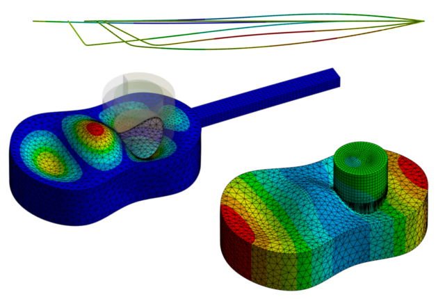
1. シミュレーション対象
アコースティックギター(acoustic guitar)は、撥弦楽器であるギターのうち、より古典的な、楽器から直接音声を伝えるものを指します。標準で6本の弦をもち、指先と爪を使って弾くフィンガーピッキング、あるいはピックではじくピック奏法で演奏され、弦の振動および音波は楽器本体および本体内の空洞の共鳴を経て奏者や聴客の耳へ届きます[1]。
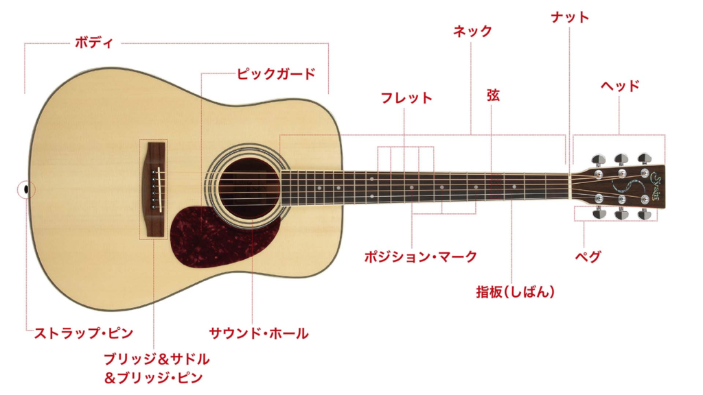
ギターの構造 参考文献[2]より引用
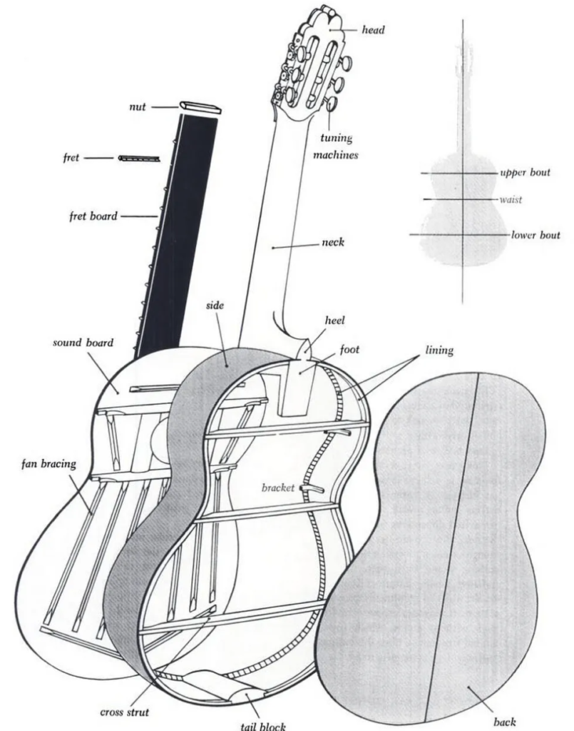
ギターの内部構造 参考文献[3]より引用
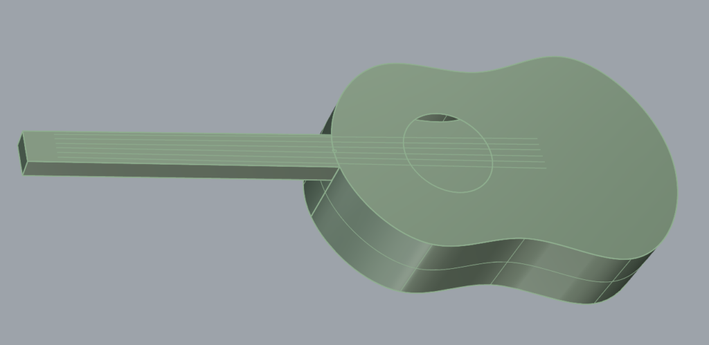
シミュレーションに使用する3Dモデルとしては、Ansysのチュートリアルページ[4]で公開されている以下のような簡単なものを使用しました。(実物で板の裏側に入っている補強のはりはモデル化されていません。)
2. 振動伝達経路の整理
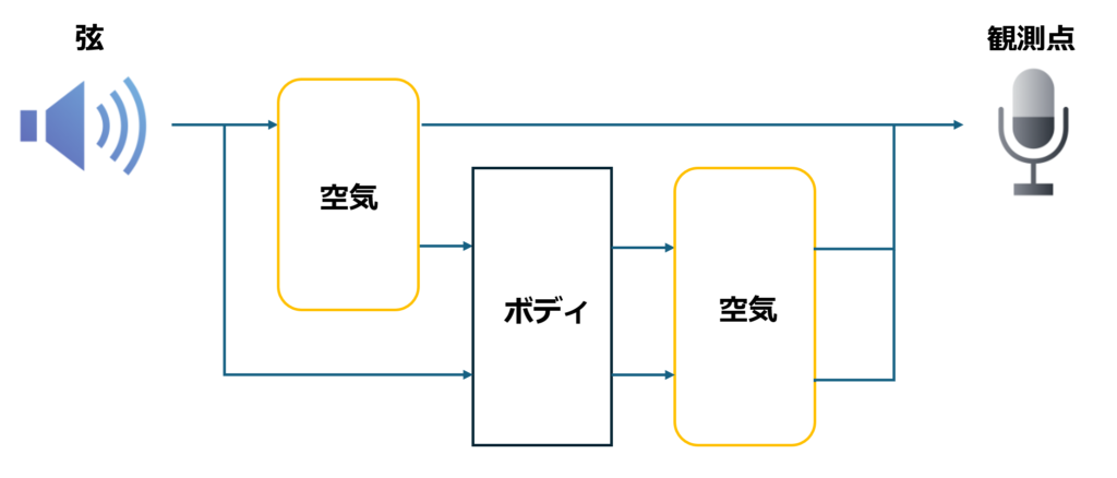
複雑な振動現象では、加振源から振動を観測する点に至るまで、振動が複雑な伝達経路をたどっていることが多く、それらをまとめて一つの問題として扱うことは非常に難しいです。そこで、振動伝達経路をしっかりと整理し、経路上の各要素単位に問題を分割して考えることが重要です。アコースティックギターでは以下のように、弾かれた弦が加振源となり、その振動が弦周辺の空気に伝播する経路と、弦とボディの接合部(ブリッジ)を通してボディに伝播する経路が考えられます。
3. 弦の振動
まずは加振源である弦単体での特性について考えます。
3.1. 背景知識(連続体力学の弦理論)
連続体力学における弦の理論から、弦には以下のような固有振動モードが存在し、撥弦時の弦の振動はこれらの固有振動モードの重ね合わせで表されます。(詳しい導出は参考文献[5]をご覧ください)
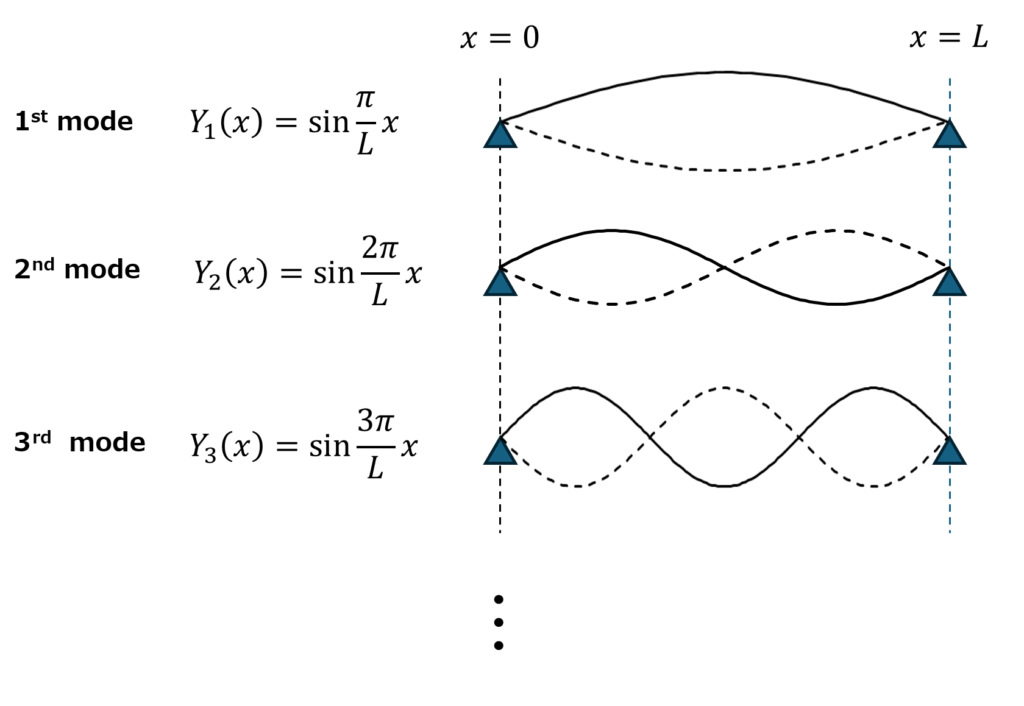
ここで、n次モードの振動数(n次固有振動数)は以下の式で表されます。
\(f_n=\frac{n}{2L}\sqrt{\frac{T}{\rho}}\)(L : 弦の長さ、T : 張力、ρ : 単位長さあたりの質量)
この式からわかる重要な性質が以下になります。
- 固有振動数はすべて1次固有振動数の整数倍になっています。この性質により弦の振動によって発生する音は単一の音程を持った音として知覚されます。1次固有振動数は基本周波数と呼ばれ、音程の高さを決定します。また、2次以降の固有振動モードから発生する音は倍音と呼ばれ、それぞれの倍音の音量の比率によって音の音色が決定します。
- 固有振動数は張力の平方根に比例します。なので、張力を大きくすると音程が上がります。
- 固有振動数は弦の長さに反比例します。なので、弦の長さを短くすると音程が上がります。
3.2. シミュレーション
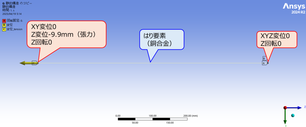
それでは弦の詳細な挙動をシミュレーションによって確認していきましょう。まずは、固有振動数解析によって固有振動モードを求めます。有限要素法で弦を扱う際に注意すべき点としては、弦に作用する張力によって弦に大変形が発生し、それによって弦の剛性が変化するという非線形現象を考慮する必要があります。なので、最初に弦に張力を静荷重として作用させる大変形ありの非線形解析を行い、求まった定常点において固有振動数解析を行います。解析のセットアップは以下になります。(強制変位の量は1次固有振動数が1弦の音程(329.6Hz、「ミ」の音)に合うよう手動チューニング)
解析結果を以下に示します。
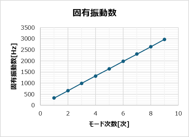
- 固有振動数一覧(9次まで)
- 固有振動モード(3次まで)
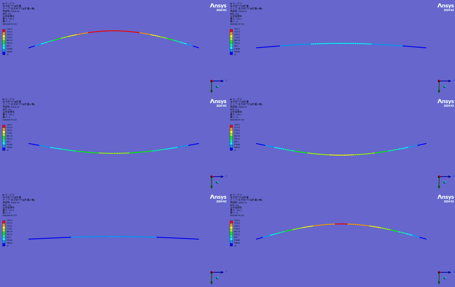
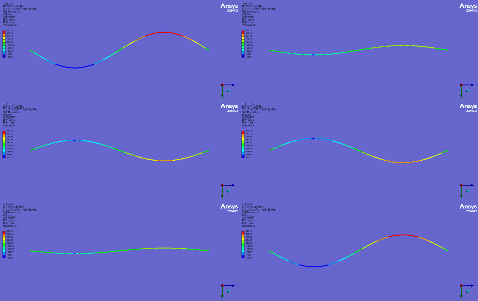
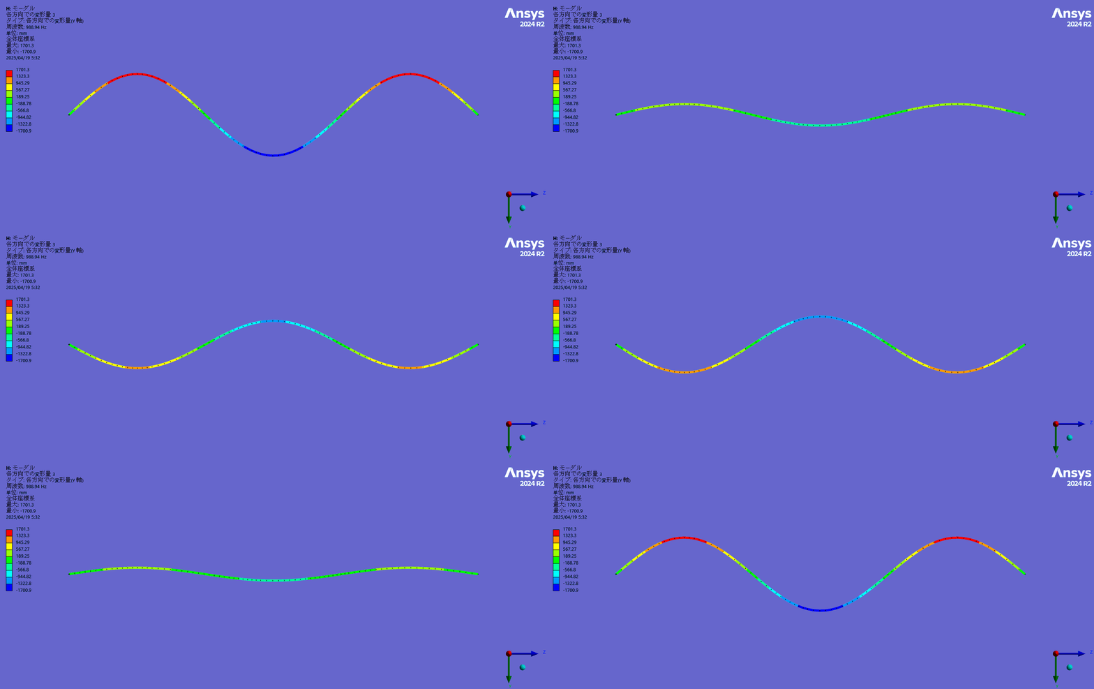
1次固有振動数は得られた張力から計算した理論値329.5Hzに近く、また、2次以降の固有振動数は基本周波数のほぼ整数倍になっており、モード形状は正弦波状になっていることが確認できました。(弦理論では弦のせん断剛性を考慮していないため固有振動数は理論値より若干高周波側にずれます。)
次に、撥弦したときの挙動を時刻歴応答解析により確認します。解析のセットアップは以下になります。撥弦は撥弦位置に強制変位を与えた状態から解放することでモデル化されます。
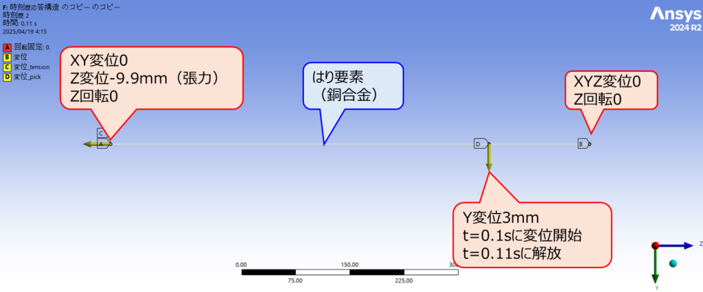
解析結果を以下に示します。
-
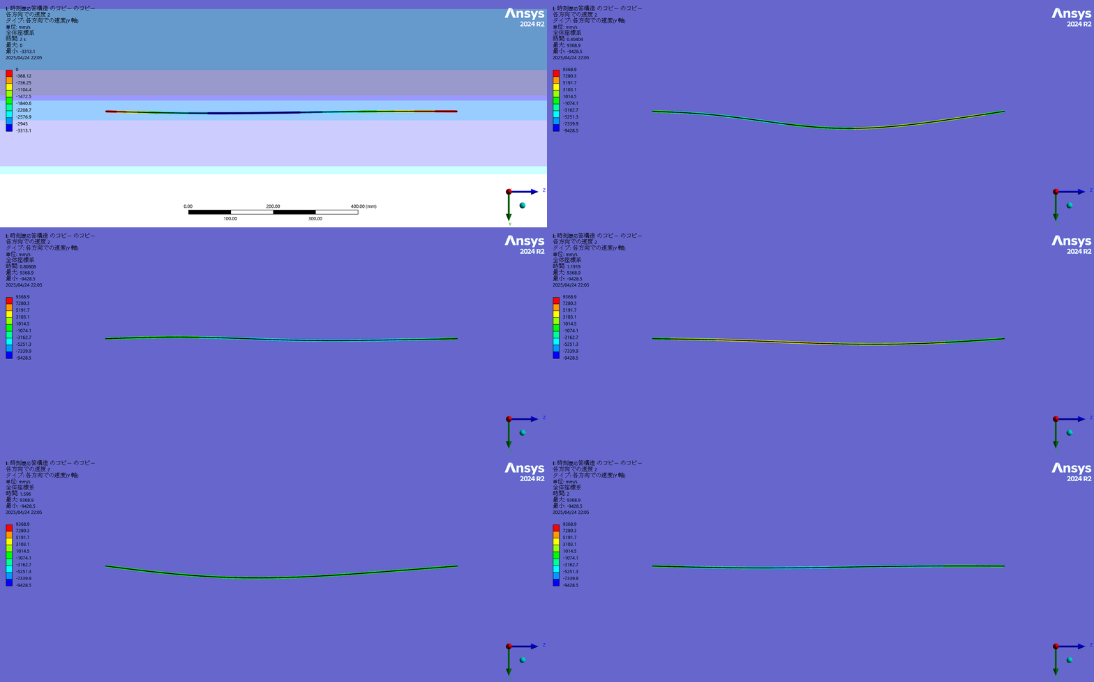
変形形状(高速で振動しているためコマ落ちしてゆっくり振動しているように見えています)
-
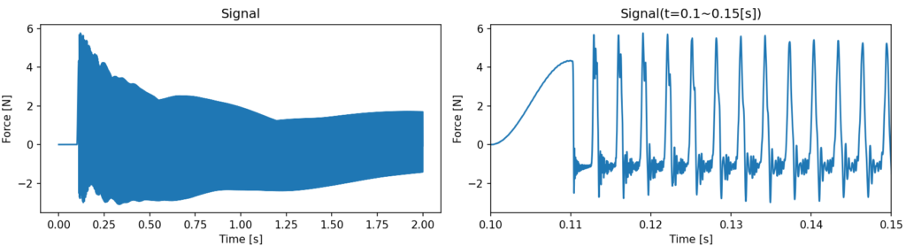
右端固定端(ブリッジ)にかかるY方向の力の時刻歴波形
-
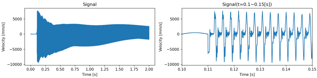
サウンドホール位置での弦の速度の時刻歴波形
-
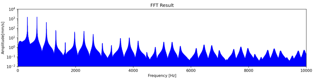
上記の速度波形をフーリエ変換することによって求めた周波数振幅特性
-
上記の速度波形を音声データとして書き出したもの
振幅特性を見ると一次固有振動数の整数倍の周波数にピークが立っていることが確認でき、聴覚的にも単一の音程を持つ音が生成されています。理論的には一次固有振動数の整数倍以外の成分は出ないですが、実際には減衰による過渡的な変化の影響で一次固有振動数の整数倍を中心にある程度幅のある周波数範囲で応答が出ます。
4. ボディ、空気の振動
次にボディ、空気を伝播する振動について考えます。
4.1. 背景知識(伝達関数)
入力波形から出力波形を生成するシステムとして線形かつ時間変化のないシステムを仮定し、そのシステムに短いパルスを入力したときの出力波形をインパルス応答と呼びます。(今回の例では入力波形がサウンドホール位置での弦の速度またはブリッジを通してボディに加わる力、出力波形が観測点での圧力変動に相当)
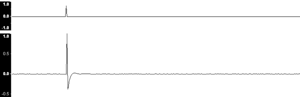
入力パルスとインパルス応答 参考文献[6]より引用
ただし、ここでいう線形とは、複数の入力波形がシステムに入ってきたときにそれぞれの影響を分けて考えることができること、入力を定数倍すると出力も定数倍されることを言います。すると、任意の入力波形について、以下のように「入力波形をパルスの足し合わせに分解⇒それぞれのパルスに対するインパルス応答を足し合わせて出力波形を得る」という操作が可能になります。
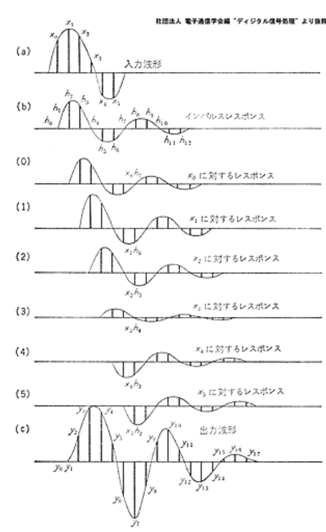
参考文献[7]より引用
すなわち、インパルス応答さえわかればそのシステムの特性がすべてわかったのと同じということになります。この操作を数式で表現すると以下のようになり、いわゆる畳み込み積分の形になります。
\(y(t)=\int^{\infty}_{-\infty} x(\tau)h(\tau-t)d\tau\) (x : 入力波形、y : 出力波形、h : インパルス応答)
この畳み込み積分には重要な性質があり、等式の両辺をフーリエ変換することで、以下の等式を得ます。
\(Y(\omega)=X(\omega)H(\omega)\) (X : 入力波形の周波数特性、Y : 出力波形の周波数特性、H : インパルス応答の周波数特性=伝達関数)
この式から、出力波形の周波数特性は入力波形の周波数特性とシステムのもつ周波数特性である伝達関数の積として表されることがわかります。また、計算コストの重い畳み込み積分をしなくとも、入力波形をフーリエ変換して伝達関数との積を計算し、その結果を逆フーリエ変換することで出力波形を得ることができるということでもあります。よって伝達関数もインパルス応答と同様にシステムの特性の全てを表していると言えます。伝達関数はある入力とそれに対する出力の例があれば、\(H(\omega)=\frac{Y(\omega)}{X(\omega)}\)により簡単に求められます。(\(X(\omega)\neq0\)である必要はあります。)
4.2. シミュレーション
それではボディ、空気の振動伝達特性をシミュレーションによって確認していきましょう。構造(ボディ)の支配方程式は運動方程式であり、音響(空気)の支配方程式はヘルムホルツ方程式であるため、構造-音響連成のマルチフィジックス問題になっていますが、多くの商用ソルバーでこういったマルチフィジックスの解析がサポートされており、特に面倒な処置もなく解析が行えるようになっています。
まずは、弦からボディに振動が伝播する経路についてシミュレーションします。解析のセットアップは以下になります。有限要素法でボディ外側の無限に広がる開空間を表現することはできないので、開空間のうち観測点周りのみをモデル化し、その端部には非物理的な音波の反射を防ぐための吸収層を配置しています。各加振周波数での応答から、伝達関数が求められます。
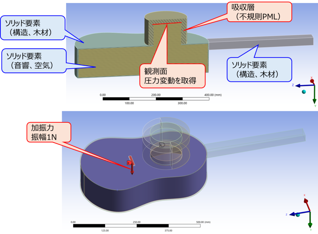
解析結果は以下になります。
-
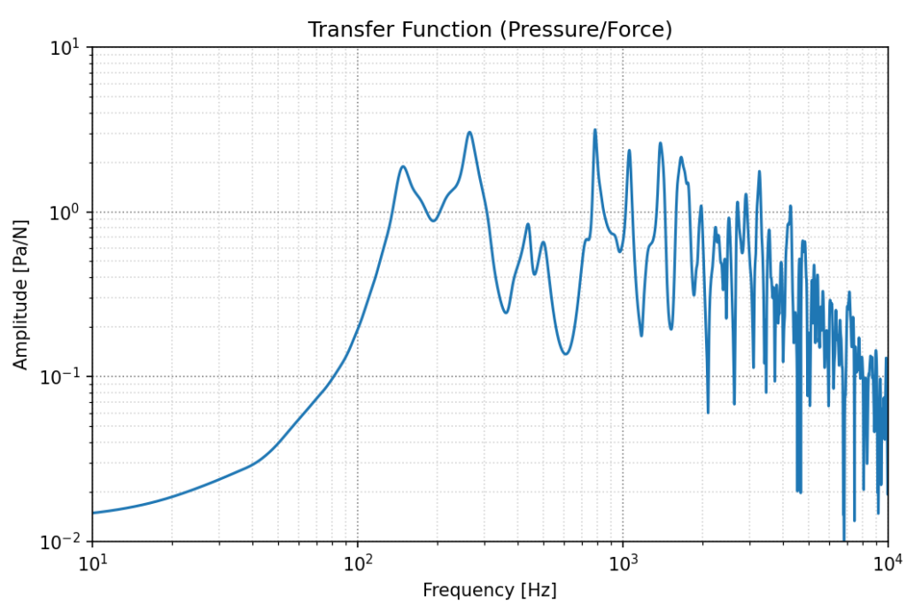
伝達関数(振幅)
-
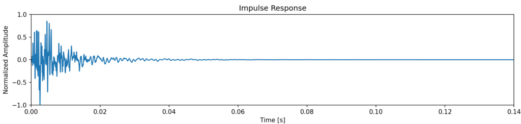
インパルス応答
-
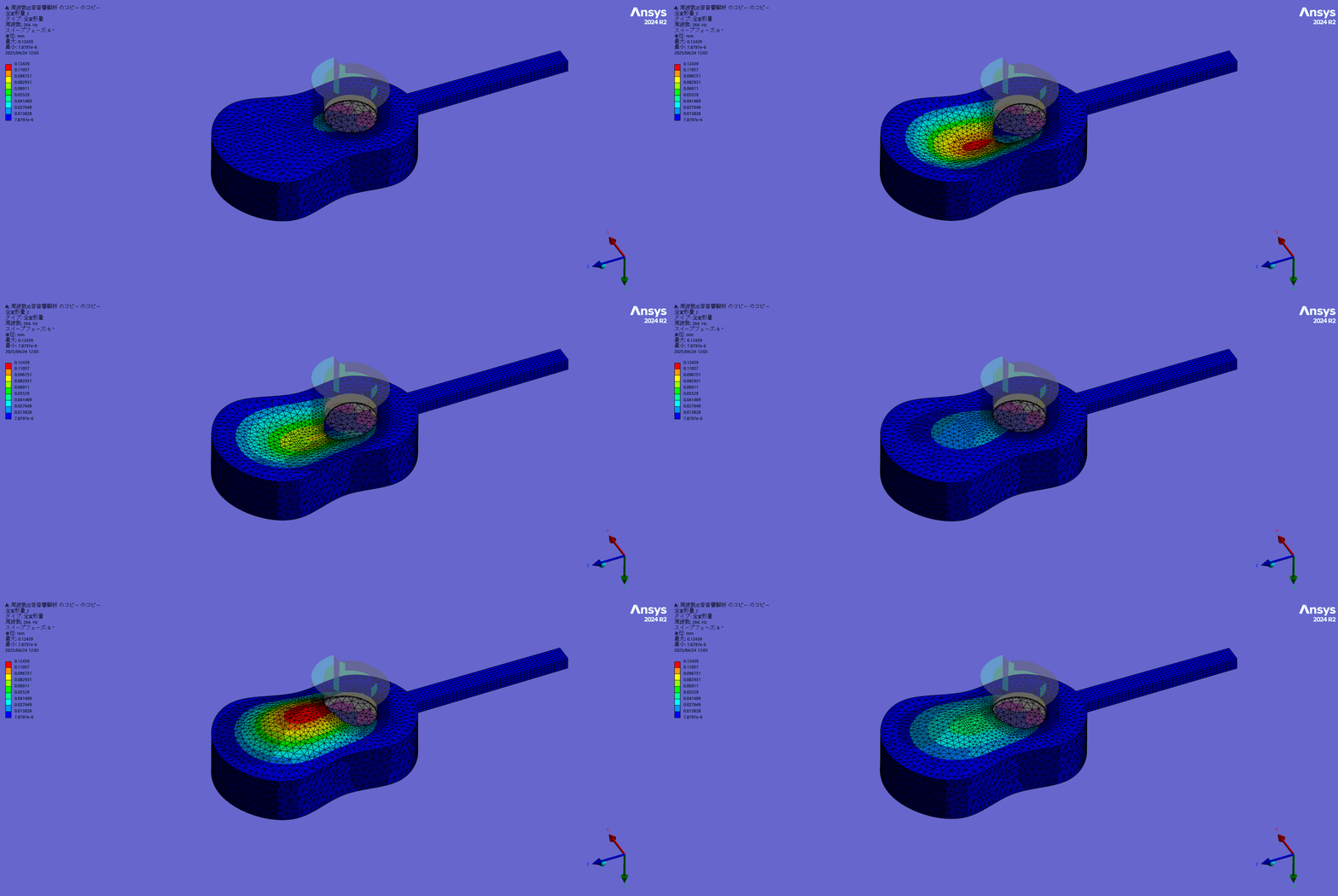
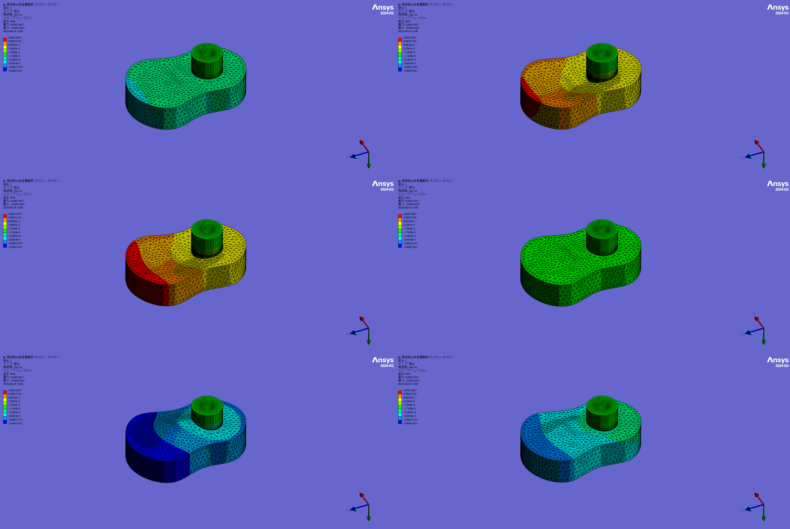
主要な応答ピーク周波数での振動の様子(ボディの変位、空気の圧力変動)
264Hz
784Hz
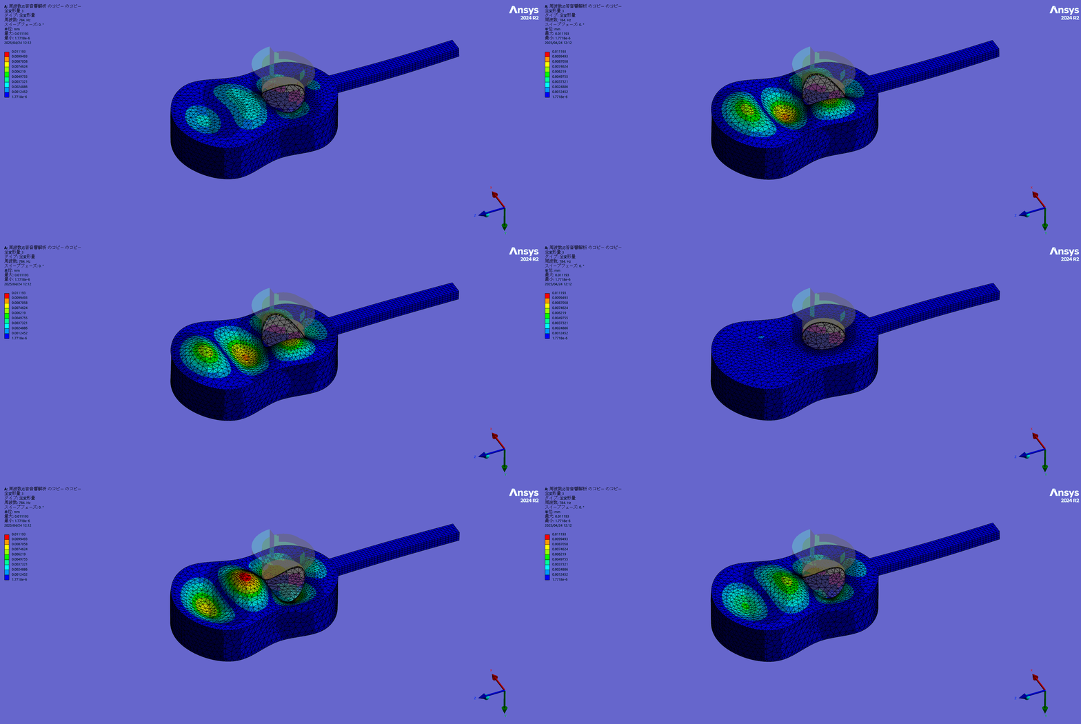
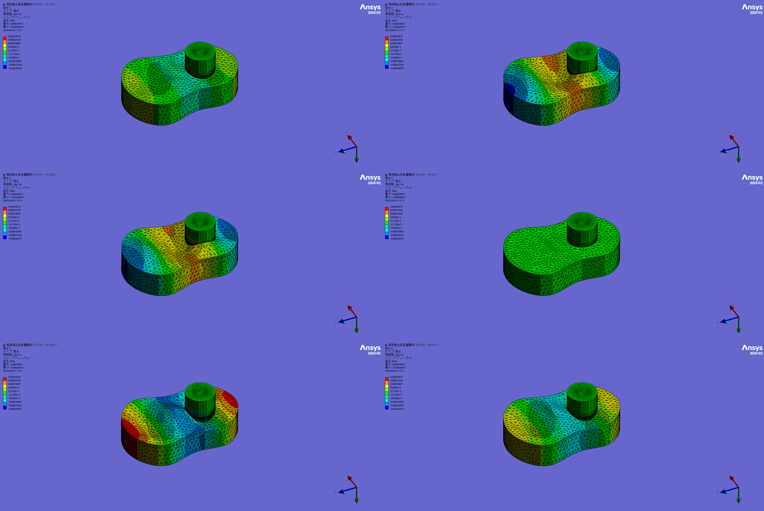
ボディ、空気ともに周波数によって異なる振動モードで振動しており、それによって伝達関数が複数の共鳴ピークを形成していることが分かります。加えて、ボディに応答性の高い振動モードのある低周波域での応答がメインであり、高周波域ではボディに応答性の高いモードがないため、応答が小さくなっています。
次に、弦から空気に振動が伝播する経路についてシミュレーションします。解析のセットアップは加振方法のみが変化し、以下のように弦を模した細長い空洞の表面に速度を与えます。
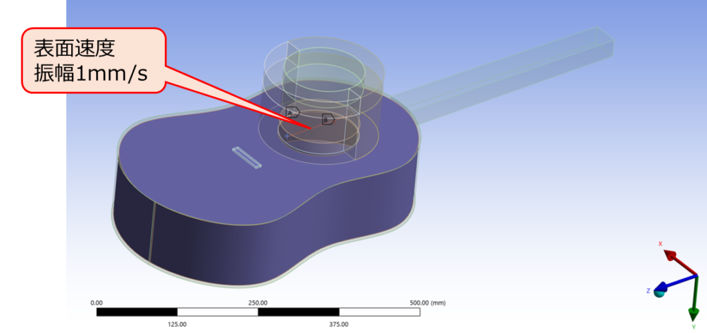
解析結果は以下になります。
-
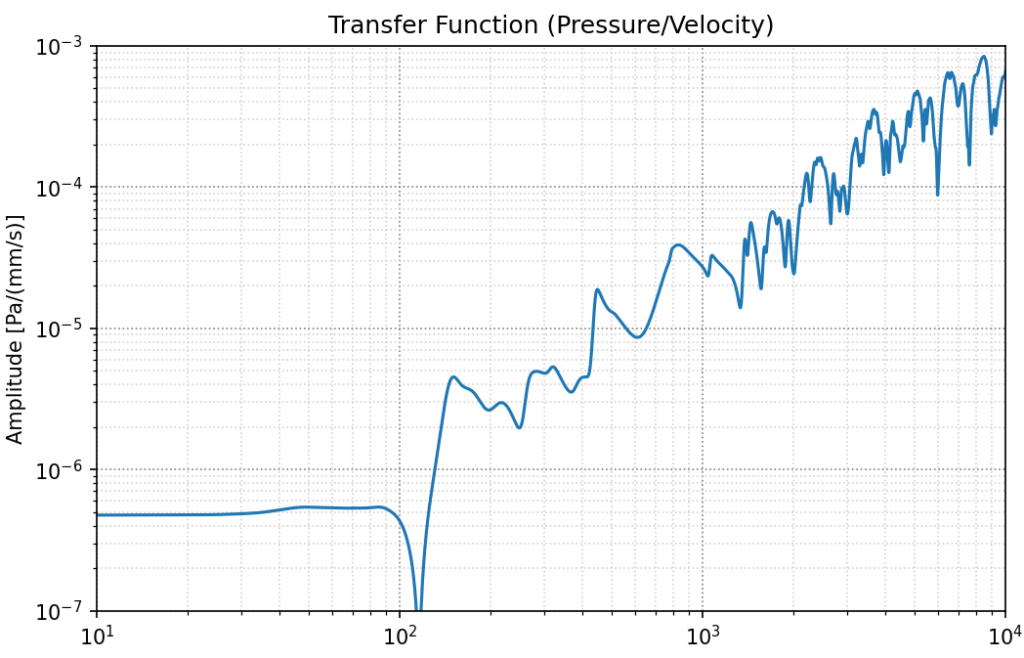
伝達関数(振幅)
-
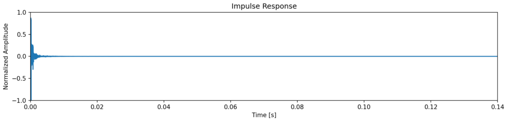
インパルス応答
-
主要な応答ピーク周波数での振動の様子(ボディの変位、空気の圧力変動)
433Hz
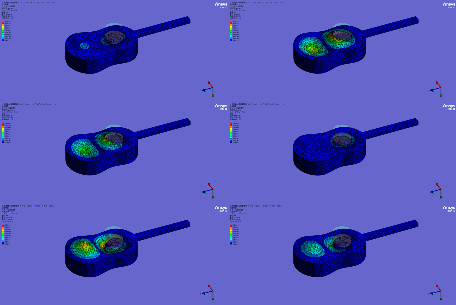
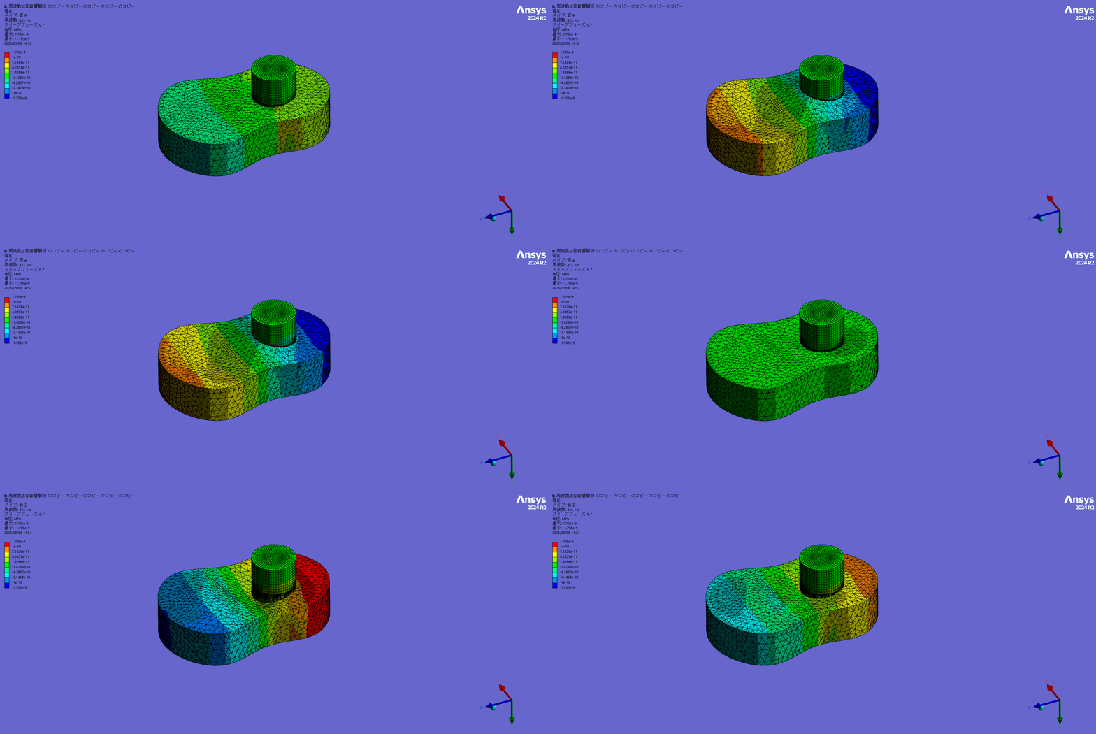
ボディ加振のときより共鳴によるピークが小さく、高周波域に向かってなだらかに応答が大きくなっていく全体的な傾向の影響が大きくなっています。
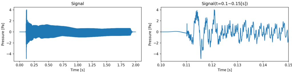
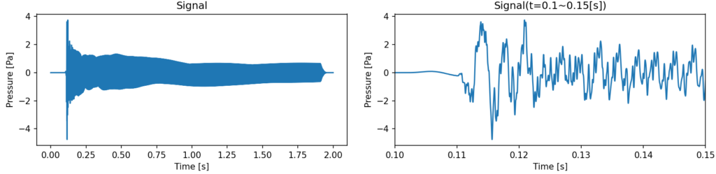
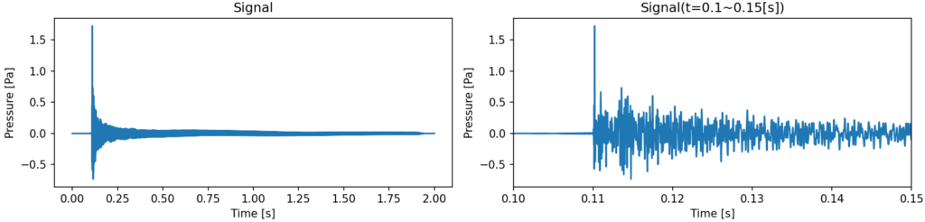
それでは最後に、この2つの伝達関数から観測点での音声波形を計算してみましょう。弦のシミュレーションで求めた固定端にかかる力の波形、サウンドホール位置での速度波形を入力とし、それぞれ周波数領域で伝達関数との積をとり、時間領域に戻し、最後に2つの圧力変動波形の和をとります。(実際には弦の運動も空気やボディの影響を受けるのですがここではその影響は無視します。)
得られた結果は以下のようになりました。
-
観測点での音
-
弦からボディに伝播する音
-
弦から空気に伝播する音
-
振幅特性の比較(ボディ伝播と空気伝播の比較、弦の速度波形と観測点の圧力波形の比較)
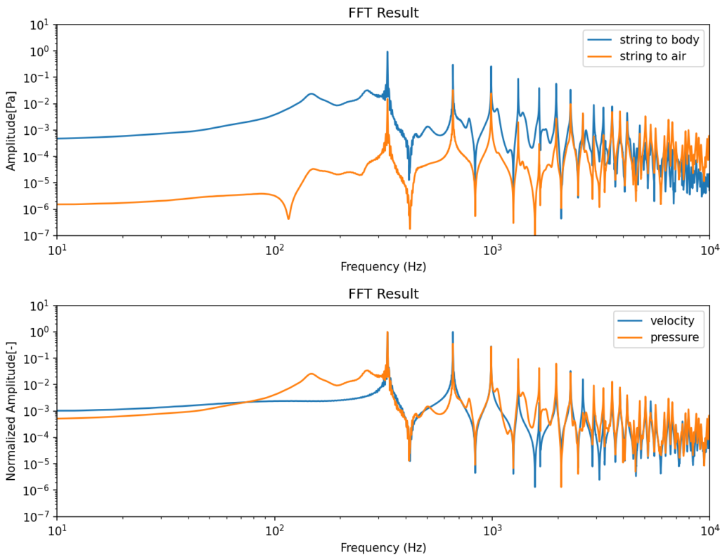
3節の純粋な速度波形に比べると、共鳴によって周波数特性が変化しギターとしての色付けがなされています。倍音の振幅比の変化の他には、減衰による過渡的な変化によってわずかに発生する非音程成分(一次固有振動数の整数倍以外の成分)が伝達経路と共鳴し、一次固有振動数の整数倍以外の周波数にピークができているのが特徴的で、それによって撥弦の直後に非音程の打撃音的なニュアンスが加わっています。また、低音~中音域の音の太さは弦からボディに伝播する音に由来していて、一方で撥弦時に特に顕著な高音域のキレは弦から空気に伝播する音に由来していることが分かります。もちろんこの伝達関数はギターの形状や材料物性によっても大きく異なり、形状設計や材料選定によって味わい深いギターの伝達関数を作りこんでいくのが設計者の仕事と言えるでしょう。
4.3. 公知の設計事例紹介
どのように伝達関数を作りこんでいくかの参考として、設計によってアコースティックギターの伝達特性を制御する例を何個か紹介しておきます。
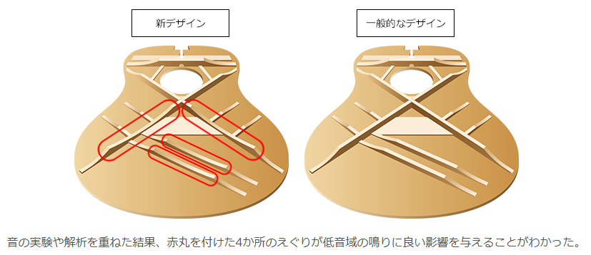
- スキャロップドブレイシング(ヤマハ等)[8]
トップ材の背面の補強材のえぐり形状を制御することで必要な強度を保ちつつ低音域の鳴りを向上させています。(もちろん補強材の配置についても強度、音響特性がよくなるように考えて設計されています。)
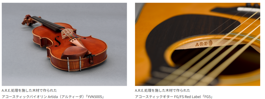
- Acoustic Resonance Enhancement技術(ヤマハ)[9]
筒状の金属製圧力容器の中に木材を入れ、内部温度、湿度を管理し、さらに段階的に圧力を変化させて処理を行うことで、木材の物性を所望のもの(楽器としての「いい音」と強度を兼ね備えたもの)に変化させる技術です。具体的には、弦の張力方向である木目方向に固くすることで弦の張力に対する強度を確保しつつ、撥弦時の振動方向である厚み方向に柔らかくすることで低音域の鳴りをよくしています。
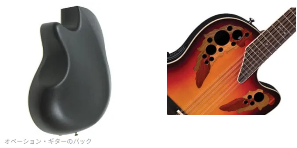
- Ovation Guitar[10]
バック材が強化プラスチックによる曲面構造になっており、ボディ内で反響した音がすべてサウンドホールに集中するようになっています。また、サウンドホールも均一でバランスの取れた音響特性を実現する、意匠面でもインパクトのある独特のものになっています。攻めた設計で独特のサウンドを作り出していてとても面白いです。
5. 奏法の再現(おまけ)
ギターの音を出力はできたものの、現状ではまだ単一の音程を鳴らすことしかできないので、ギターの奏法も再現してみましょう。
5.1. 押弦
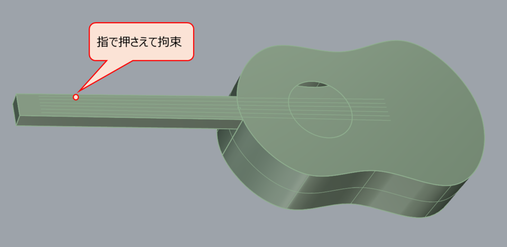
指で弦を指板に押し付けることで拘束し弦の有効長を変化させ、固有振動数を変化させることで様々な音程で音を鳴らすことができるようになります。
ここでは、1弦の「ミ」音を押弦によって「シ」音に変化させてみましょう。まず、平均律と呼ばれる最も一般的な音階の定義は以下になります。
- 1オクターブ上になると周波数が2倍になる
- 1オクターブの中に12種類の音がある(ド、ド#、レ、レ#、ミ、ファ、ファ#、ソ、ソ#、ラ、ラ#、シ)
- 音階上で隣り合った音同士の周波数比は常に一定
- 真ん中の「ラ」音の周波数を440Hzと定義
すなわち、真ん中の「ラ」音よりn個上の音の周波数は\(440\times2^{\frac{n}{12}}\)[Hz]と表されます。(nが負でも同じ)
ここで、「ミ」音に対して「シ」音は7個上の音なので周波数比は\(2^{\frac{7}{12}}=1.498\)倍になります。なので、弦理論の式から、弦の長さを\(\frac{1}{1.498}=0.667\)倍にする点で押弦すればよいことになります。実際には、押弦時の張力増加を考慮して弦の長さを若干長めにします。参考文献[8]によると弦の長さを理論値に対し\(\frac{1}{0.995}=1.005\)倍にするのがよいそうです。
解析では、押弦する点にXY変位拘束を与えます。(X方向は変位0、Y方向は弦から指板までの距離だけ変位させる)
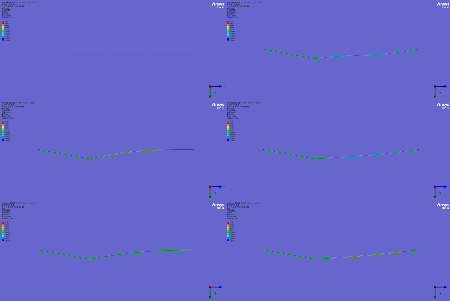
解析結果(弦の変形形状、音声データ)は以下になります。また、1次固有振動数は492.6Hzであり、音程の定義値493.9Hzに近い値になっていました。
5.2. コード(和音)
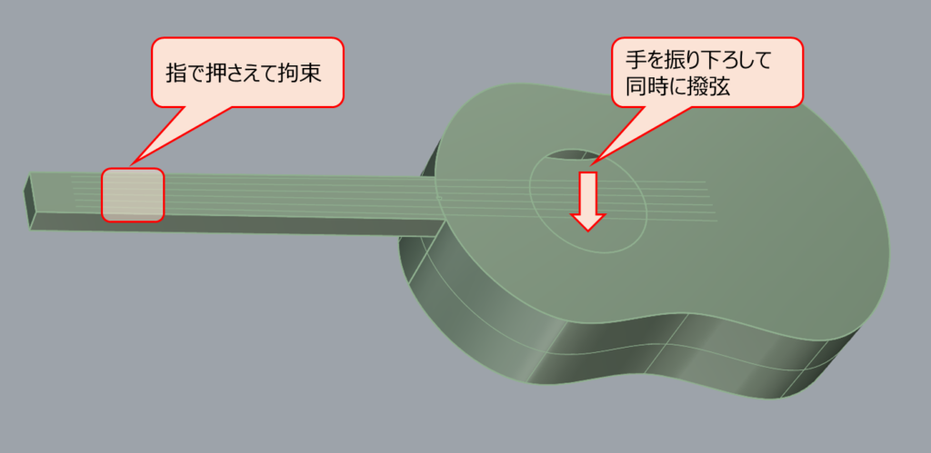
押弦によって複数の弦の固有振動数を調整し、手を振り下ろして同時に撥弦することでコード(和音)を鳴らすことができます。これで最低限の演奏はできるようになります。
ここでは、例としてCメジャーコード(ド、ミ、ソ)を弾いてみましょう。メジャーコードは構成音の周波数比がほぼ4:5:6ときれいな整数比で表せるコードで、調和した響きとして知覚されます。(逆に言うと、このように音階から規則的に音を選んで作った和音がきれいな整数比で響くように音階の定義を決めたというわけです。)
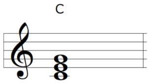
このコードをギターで鳴らす際のルールが以下になります。(オクターブ違いは同じ音として扱います)
- 全ての弦においてコードの構成音のどれかを鳴らす
- コードの構成音がすべて少なくとも1本以上の弦で鳴らされている
- 一番低音側の弦ではベース音(Cメジャーコードならド)を鳴らす
また、1弦から6弦までの最も一般的なチューニングは以下になります。(音名の数字はオクターブ違いを区別しています)
| 弦 | 音名 | 周波数 |
|---|---|---|
| 1弦 | ミ4 | 329.6Hz |
| 2弦 | シ3 | 246.9Hz |
| 3弦 | ソ3 | 196.0Hz |
| 4弦 | レ3 | 146.8Hz |
| 5弦 | ラ2 | 110.0Hz |
| 6弦 | ミ2 | 82.4Hz |
これらを考慮すると、押弦の仕方の一例はこのようになります。音程は1弦から順にミ4、ド4、ソ3、ミ3、ド3です。(6弦は弾かない)

今回のモデルでは弦同士の相互作用はないので1本ずつ計算して足し合わせても同じになりますが、実際には弦同士の間で共振が起こります。(例えばド3の3次固有モードとソ3の2次固有モードは固有振動数がほぼ同じであるため共振します。)そこで、他の弦の波形を指数関数的に減衰させて作成したインパルス応答を元波形と畳み込むことで共鳴成分を近似し、元波形に薄く足し合わせることにします。
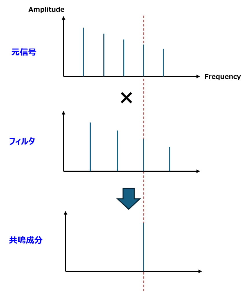
また、手を振り下ろすことで低音弦から順番に弾かれていくので、強制変位を与えるタイミングを少しずつずらします。
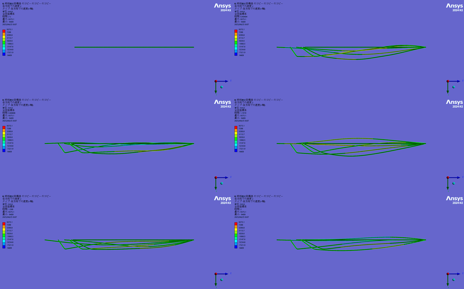
解析結果(弦の変形形状、観測点での音)は以下になります。
長くなってしまったのでここでは触れませんが、ギターにはこの他にもまだまだ多彩な奏法があり、物理的な観点でも面白いものも多いです!
6.まとめ
今回はギターのシミュレーションを通して、振動・音響問題の考え方や、ギターの発音メカニズムについて説明しました。音楽を聴くときは、その背後にある物理にまで思いを馳せてみるとより音楽を楽しめるのではないかと思います。
参考文献
[2]https://acousticguitarmagazine.jp/beginners/2024-0510-parts-name/
[3]https://ja.namu.wiki/w/클래식 기타/재료 및 구조
[5]https://ds.cc.yamaguchi-u.ac.jp/~tsaito/D02/DynamicsII11.html
[6]https://ja.wikipedia.org/wiki/%E3%82%A4%E3%83%B3%E3%83%91%E3%83%AB%E3%82%B9%E5%BF%9C%E7%AD%94
[7]https://www.noe.co.jp/technology/18/18inv1.html
[8]https://jp.yamaha.com/sp/myujin/11120.html
[9]https://www.yamaha.com/ja/tech-design/research/technologies/are/
[10]https://nihon-meisho.com/144/
[11]http://www.crane.gr.jp/MakingGuitarZero/CRANE_027_01flet_formalize.html
1. simulation object
The acoustic guitar is the more classical version of the guitar, a stringed instrument that transmits sound directly from the instrument. It has six standard strings and is played by fingerpicking or plucking with a pick. The vibrations of the strings and sound waves reach the ears of the player and audience through the resonance of the body of the instrument and the cavities inside the body [1].
Structure of a guitar Adapted from Reference [2]
<img src=“https://nature-architects.com/wp-content/uploads/2025/05/image-12-805x1024.png” alt=“” width=“402” height=“612” class="size- large wp-image-2455” />
Internal Structure of a Guitar Adapted from Reference [3]
For the 3D model used in the simulation, we used the following simple model from the Ansys tutorial page [4]. (The reinforcing beams that are in the backside of the board in the real one are not modeled.)
2. Organizing vibration transmission paths
In complex vibration phenomena, vibration often follows complicated transmission paths from the excitation source to the point where the vibration is observed, and it is very difficult to treat them all together as a single problem. Therefore, it is important to organize the vibration transmission path and divide the problem into units for each element on the path. In the case of an acoustic guitar, as shown below, there are two possible paths: the path where the plucked string is the excitation source and its vibration propagates to the air around the string and the path where it propagates to the body through the junction between the string and the body (bridge).
3. string vibration
First, we consider the properties of the excitation source, the string by itself.
3.1. Background knowledge (string theory in continuum mechanics)
According to the theory of strings in continuum mechanics, strings have the following eigenfrequency modes, and the vibration of a string during string repulsion is represented by the superposition of these eigenfrequency modes. (For a detailed derivation, see reference [5])
!
Here, the frequency of the nth-order mode (nth-order natural frequency) is expressed by the following equation.
\(f_n=\frac{n}{2L}\sqrt{\frac{T}{\rho}}\)
(L : length of string, T : tension, ρ : mass per unit length)
The important properties that can be found from this equation are as follows.
- All natural frequencies are integer multiples of the first-order natural frequency. The first natural frequency is called the fundamental frequency and determines the pitch of the sound. The sounds produced by the second and subsequent eigenfrequency modes are called overtones, and the timbre of the sound is determined by the ratio of the volume of each overtone.
- The natural frequency is proportional to the square root of tension. Therefore, increasing the tension raises the pitch of the note.
- The natural frequency is inversely proportional to the length of the string. Therefore, shortening the length of the string will raise the pitch.
3.2. Simulation
Let us now check the detailed behavior of the string by simulation. First, the eigenfrequency analysis is used to obtain the eigenfrequency modes. It is important to note that when we treat strings using the finite element method, we need to take into account the nonlinear phenomenon that the tension acting on the string causes a large deformation of the string, which in turn changes the stiffness of the string. Therefore, we first perform a nonlinear analysis with large deformation where the tension is applied to the string as a static load, and then perform a natural frequency analysis at the obtained stationary point. The analysis setup is as follows (The amount of forced displacement is manually tuned so that the first natural frequency matches the pitch of the first string (329.6 Hz, “mi” note))
The analysis results are shown below.
- List of natural frequencies (up to 9th order)
- Natural Vibration Modes (up to 3rd order)
<img src=“https://nature-architects.com/wp-content/uploads/2025/05/新規-2.gif” alt=“” width=“379” height=“159” class="size-full wp-image- 2459“ /><img src=”https://nature-architects.com/wp-content/uploads/2025/05/新規-3.gif“ alt=”“ width=”379“ height=”159“ class=”size-full wp- image-2459“ /><img src=”https://nature-architects.com/wp-content/uploads/2025/05/新規-4.gif“ alt=”“ width=”379“ height=”159“ class=”size- full wp-image-2459” />
The first-order natural frequency is close to the theoretical value of 329.5 Hz calculated from the obtained tension, and the second-order and subsequent natural frequencies are almost an integer multiple of the fundamental frequency, confirming that the mode shape is sinusoidal. (The natural frequency is slightly higher than the theoretical value because string theory does not take into account the shear stiffness of the string.)
Next, we will check the behavior of the string when it is repelled by a time history response analysis. The analysis setup is as follows. The repelling string is modeled by releasing the string from a state of forced displacement at the repelling position.
The analysis results are shown below.
-
Deformation Shape (The vibration is occurring at a high speed, so the frame drops and the vibration looks like it is occurring slowly.)
-
Time history waveform of force in Y direction applied to the right fixed end (bridge)
-
Time waveform of string velocity at soundhole position
-
Frequency amplitude characteristics obtained by Fourier transforming the above velocity waveforms
-
The above velocity waveform written out as audio data
The amplitude characteristics confirm that the peak is at an integer multiple of the primary eigenfrequency, and a single pitch sound is produced aurally. Theoretically, no components other than integer multiples of the primary natural frequency are produced, but in practice, the response is produced over a frequency range with some width centered on integer multiples of the primary natural frequency due to transient changes caused by damping.
4 Body and air vibration
Next, we consider vibrations propagating through the body and air.
4.1. Background knowledge (transfer function)
Assuming a linear and time-invariant system that generates an output waveform from an input waveform, the output waveform when a short pulse is input to the system is called the impulse response. (In this example, the input waveform corresponds to the velocity of the string at the soundhole position or the force applied to the body through the bridge, and the output waveform corresponds to the pressure variation at the observation point.)
Input pulse and impulse response Adapted from reference [6].
However, linear here means that when multiple input waveforms enter the system, the effects of each can be considered separately, and that if the input is multiplied by a constant, the output is also multiplied by a constant. Then, for any input waveform, the following operation is possible: “decompose the input waveform into an addition of pulses ⇒ add the impulse responses to each pulse to obtain the output waveform.
Adapted from reference [7]
In other words, it is the same as knowing all the characteristics of the system if only the impulse response is known. This operation can be expressed in a mathematical expression as follows, which is a form of so-called convolution integral.
\(y(t)=\int^{\infty}_{-\infty} x(\tau)h(\tau-t)d\tau\)
(x : input waveform, y : output waveform, h : impulse response)
This convolution integral has an important property: by Fourier transforming both sides of the equality, we obtain the following equality.
\(Y(\omega)=X(\omega)H(\omega)\)
(X : frequency response of input waveform, Y : frequency response of output waveform, H : frequency response of impulse response = transfer function)
From this formula, it can be seen that the frequency response of the output waveform is expressed as the product of the frequency response of the input waveform and the transfer function, which is the frequency response of the system. It also means that the output waveform can be obtained by Fourier transforming the input waveform, calculating the product of the input waveform and the transfer function, and then inverting the result by Fourier transform. Therefore, it can be said that the transfer function, like the impulse response, represents all of the system's characteristics. The transfer function can be easily obtained by H=Y/X given an example input and its output. (X must not be zero.)
4.2. Simulation
Let us now check the vibration transfer characteristics of the body and air by simulation. Since the governing equation for the structure (body) is the equation of motion and the governing equation for the acoustics (air) is the Helmholtz equation, this is a multi-physics problem with structure-acoustics coupling. The first step is to analyze the vibration from the string to the body.
First, we will simulate the path of vibration propagation from the strings to the body. The analysis setup is as follows Since the finite element method cannot represent the infinite open space outside the body, only the area around the observation point is modeled out of the open space, and an absorbing layer is placed at the edge of the open space to prevent non-physical sound wave reflection. From the response at each excitation frequency, the transfer function is obtained.
The results of the analysis are shown below.
-
Transfer function (amplitude)
-
Impulse response
-
Vibration at major response peak frequencies (body displacement, air pressure fluctuations)
264Hz
<img src=“https://nature-architects.com/wp-content/uploads/2025/05/新規-6.gif” alt=“” width=“506” height=“226” class="size-full wp-image- 2479“ /><img src=”https://nature-architects.com/wp-content/uploads/2025/05/新規-7.gif“ alt=”“ width=”506“ height=”226“ class=”size-full wp- image-2479” />
784Hz
<img src=“https://nature-architects.com/wp-content/uploads/2025/05/新規-8.gif” alt=“” width=“506” height=“226” class="size-full wp-image- 2479“ /><img src=”https://nature-architects.com/wp-content/uploads/2025/05/新規-9.gif“ alt=”“ width=”506“ height=”226“ class=”size-full wp- image-2479” />
It can be seen that both the body and the air vibrate with different vibration modes depending on the frequency, which causes the transfer function to form multiple resonance peaks. In addition, the main response is in the low frequency range where the body has a highly responsive vibration mode, and the response is smaller in the high frequency range because the body does not have a highly responsive mode.
Next, we simulate the path of vibration propagation from the strings to the air. Only the method of excitation is varied in the analysis setup, and the velocity is applied to the surface of an elongated cavity that mimics a string as follows.
The results of the analysis are as follows
-
Transfer function (amplitude)
-
Impulse response
-
Vibration at major response peak frequencies (body displacement, air pressure fluctuations)
433Hz
<img src=“https://nature-architects.com/wp-content/uploads/2025/05/新規-10.gif” alt=“” width=“506” height=“226” class="size-full wp-image- 2479“ /><img src=”https://nature-architects.com/wp-content/uploads/2025/05/新規-11.gif“ alt=”“ width=”506“ height=”226“ class=”size-full wp -image-2479” />
The peaks due to resonance are smaller than with body excitation, and the overall tendency of the response to increase gently toward the high frequency range is more influential.
Finally, let us calculate the speech waveform at the observation point from these two transfer functions. We take as input the force waveform at the fixed end and the velocity waveform at the soundhole position, both obtained from the string simulation, and product each with the transfer function in the frequency domain, then back in the time domain, and finally sum the two pressure fluctuation waveforms. (In reality, the string motion is also affected by the air and the body, but we ignore that effect here.)
The results obtained were as follows
-
Sound at the observation point
-
Sound propagating from the strings to the body
-
Sound propagating from the strings to the air
-
Comparison of amplitude characteristics (body propagation vs. air propagation, string velocity waveform vs. pressure waveform at observation point)
Compared to the pure velocity waveform in section 3, the frequency characteristics are changed by resonance and colored as a guitar. In addition to the change in the amplitude ratio of the overtone, the characteristic feature is that the non-pitched components (components other than integer multiples of the primary natural frequency) generated slightly by transient changes due to decay resonate with the transmission path, creating a peak at a frequency other than integer multiples of the primary natural frequency, which adds a non-pitched strike-like nuance immediately after the plucked string. This gives the strings a non-pitched percussive nuance immediately after the plucked strings. The thickness of the sound in the low to middle register comes from the sound propagated from the strings to the body, while the sharpness in the upper register, which is particularly noticeable when the strings are plucked, comes from the sound propagated from the strings to the air. Of course, this transfer function varies greatly depending on the shape and material properties of the guitar, and it is the designer's job to create a transfer function for the guitar that is pleasing to the ear through shape design and material selection.
- Scalloped bracing (Yamaha, etc.)[8].
By controlling the gouge shape of the reinforcement on the back of the top material, the sound in the bass range is improved while maintaining the necessary strength. (Of course, the placement of the reinforcement is also designed to improve strength and acoustic characteristics.)
- Acoustic Resonance Enhancement Technology (Yamaha)[9].
This is a technology to change the physical properties of wood to the desired ones (“good sound” and strength as a musical instrument) by placing the wood in a cylindrical metal pressure vessel, controlling the internal temperature and humidity, and further processing the wood by changing the pressure in stages. Specifically, the wood is hardened in the grain direction, which is the direction of string tension, to ensure strength against string tension, and softened in the thickness direction, which is the direction of vibration when the strings are plucked, to improve the sound in the bass register.
- Ovation Guitar[10].
The back material is made of reinforced plastic with a curved surface structure, so that all the sound reverberated in the body is concentrated in the sound hole. The sound hole is also unique and impactful in terms of design, achieving uniform and balanced acoustic characteristics. The aggressive design creates a unique sound that is very interesting.
5. reproduction of playing technique (extra)
Although we have been able to output guitar sounds, we can still only play a single pitch, so let's try to reproduce the guitar's playing technique as well.
5.1. push strings
By pressing the string against the fingerboard with the fingers, we can constrain and change the effective length of the string, and by changing the natural frequency, we can make notes sound at various pitches.
Here, let's change the “mi” note on the first string to a “si” note by pressing the string. First, here is the definition of the most common musical scale, called the mean scale
- The frequency doubles as you go up an octave.
- There are 12 different notes within an octave (do, do#, re, re#, mi, fa, fa#, so, so#, la, la#, si)
- The frequency ratio between adjacent notes on the scale is always constant
- The frequency of the middle “la” note is defined as 440 Hz.
That is, the frequency of the note n above the middle “la” note is expressed as 440*2^(n/12)[Hz]. (same if n is negative)
Here, the frequency ratio is 2^(7/12)=1.498 times higher than the mi note because the si note is 7 notes higher. Therefore, from the string theory formula, it is sufficient to push the string at the point where the string length is 1/1.498=0.667 times the length of the string. In practice, the string length should be slightly longer to account for the increase in tension during pressing. According to reference [8], the string length should be 1/0.995=1.005 times the theoretical value.
In the analysis, XY displacement constraints are given to the point where the string is to be pushed. (The displacement in the X direction is 0, and in the Y direction the displacement is the distance from the string to the fingerboard)
The analysis results (deformed shape of the string and sound data) are shown below. The first-order natural frequency was 492.6 Hz, which is close to the pitch definition value of 493.9 Hz.
5.2. chords
By adjusting the natural frequencies of several strings by pressing them, and then simultaneously plucking them by swinging the hand down, chords can be played. This will allow you to play at a minimum.
Let's play a C major chord (do, mi, so) as an example. A major chord is a chord in which the frequency ratio of the component notes can be expressed in a neat integer ratio of approximately 4:5:6, and is perceived as a harmonic sound. (Conversely, the definition of the scale was determined so that chords made by regularly selecting notes from the scale like this would sound in a clean integer ratio.)
The rules for sounding this chord on the guitar are as follows. (Octave differences are treated as the same note.)
- Play any of the chord's component notes on all strings.
- Every note of the chord is played on at least one string.
- The bass note (Do for a C major chord) is sounded on the lowest string.
Also, the most common tunings for strings 1 through 6 are as follows (The numbers in the note names distinguish octave differences.)
| String | Note | Frequency |
|---|---|---|
| 1 | mi4 | 329.6Hz |
| 2 | si3 | 246.9Hz |
| 3 | so3 | 196.0Hz |
| 4 | re3 | 146.8Hz |
| 5 | la2 | 110.0Hz |
| 6 | mi2 | 82.4Hz |
Considering these factors, an example of how to push the strings would look like this. The pitches are, starting from the 1st string, mi4, do4, so3, mi3, do3. (the 6th string is not played)
In this model, there is no interaction between the strings, so if we calculate them one by one and add them together, they will be the same, but in reality, resonance will occur between the strings. (For example, the third-order eigenmode of Do 3 and the second-order eigenmode of So 3 resonate because their eigenfrequencies are almost the same.) Therefore, we approximate the resonance component by convolving the impulse response created by exponentially damping the waveforms of the other strings with the original waveform, and add it thinly to the original waveform.
<img src=“https://nature-architects.com/wp-content/uploads/2025/05/image-44-846x1024.png” alt=“” width=“423” height=“512” class="size- large wp-image-2509” />
In addition, the timing of the forced displacement is shifted slightly as the strings are plucked in order from the bass strings by swinging the hand down.
The results of the analysis (deformed shape of the string and sound at the observation point) are as follows.
This is too long to go into here, but the guitar still has many other varied techniques, many of which are interesting from a physical standpoint as well!
6. Summary
In this article, we have explained the concept of vibration/acoustic problems and the pronunciation mechanism of the guitar through guitar simulations. When listening to music, I think you will enjoy music more if you think about the physics behind it.
References.
[1]https://ja.wikipedia.org/wiki/%E3%82%A2%E3%82%B3%E3%83%BC%E3%82%B9%E3%83%86%E3%82%A3%E3%83%83%E3%82%AF%E3%83%BB%E3%82%AE%E3%82% BF%E3%83%BC
[2]https://acousticguitarmagazine.jp/beginners/2024-0510-parts-name/
[3][https://ja.namu.wiki/w/클래식 기타/재료 및 구조](https://ja.namu.wiki/w/%ED%81%B4%EB%9E%98%EC%8B%9D%20%EA%B8%B0%ED%83%80/%EC%9E%AC%EB%A3%8C %20%EB%B0%8F%20%EA%B5%AC%EC%A1%B0)
[4]https://innovationspace.ansys.com/courses/courses/large-deformation/lessons/homework-quizzes-simulation-examples-large- deformation-in-structural-mechanics-lesson-5/
[5]https://ds.cc.yamaguchi-u.ac.jp/~tsaito/D02/DynamicsII11.html
[6]https://ja.wikipedia.org/wiki/%E3%82%A4%E3%83%B3%E3%83%91%E3%83%AB%E3%82%B9%E5%BF%9C%E7%AD%94
[7]https://www.noe.co.jp/technology/18/18inv1.html
[8]https://jp.yamaha.com/sp/myujin/11120.html
[9]https://www.yamaha.com/ja/tech-design/research/technologies/are/
[10]https://nihon-meisho.com/144/
[11]http://www.crane.gr.jp/MakingGuitarZero/CRANE_027_01flet_formalize.html
