
0. はじめに
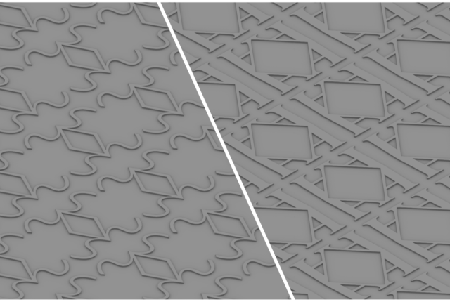
弊社では、ある機能条件が与えられた際に、さまざまな最適化手法を駆使して構造形状を設計しています。それぞれの手法には長所と短所があり、問題設定やパラメータの調整、手法の組み合わせなど、多くの工夫と試行錯誤が必要とされます。
一方で、近年、深層学習(DL; Deep Learning)を用いた生成技術の発展はめざましく、入力指示に従って文章や画像を自動生成することが当たり前になりつつあります。
もし、DLを用いて、条件から直接構造形状を導出できる生成モデルが実現できれば、こうした試行錯誤を省略でき、設計業務が非常に効率化されることでしょう。はたして、設計の分野においても、条件を入力するだけで適切な形状が得られるような生成モデルは実現可能なのでしょうか。
1. 生成モデルについて
生成モデルは、学習データに基づき「もっともらしい」新たなデータをに生成します。
深層ニューラルネットワークを用いた生成モデルも多数種類がありますが、今回は筆者の理解と実装が最も早かった敵対的生成ネットワーク(GAN; Generative Adversarial Network)を採用しました。
GANは生成器(Generator)と識別子(Discriminator)という2つのニューラルネットワークを互いに競わせながら学習を行うことで、学習データに類似した画像を生成することができるようになります。明瞭な境界が得られやすく、高速に生成できる点が主な利点です。
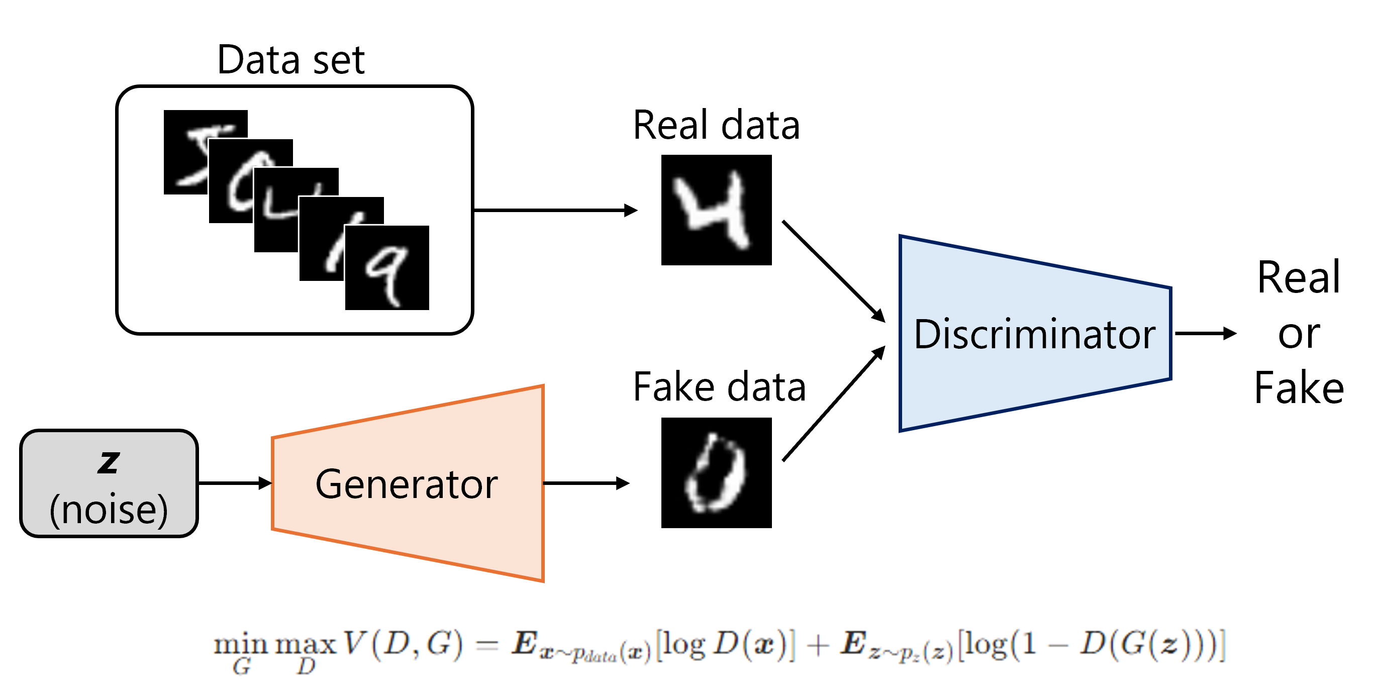
標準的なGANでは、出力される画像はランダムノイズに依存するため、生成結果を制御することができません。
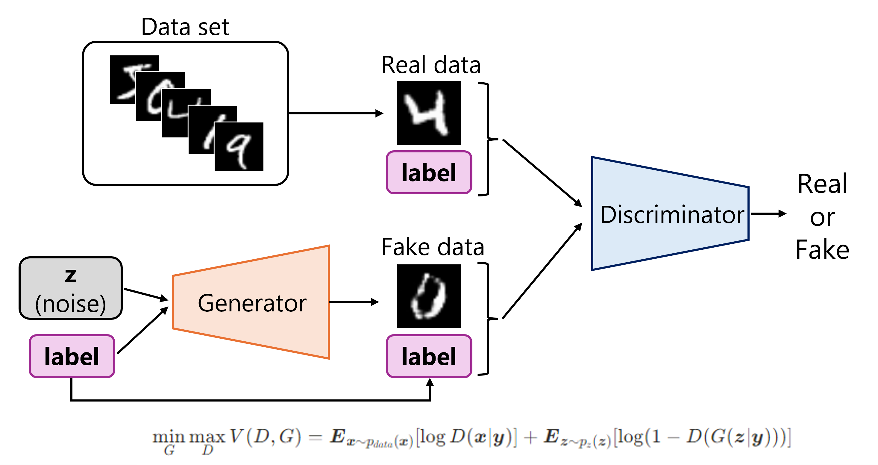
そこで、条件付きGAN(Conditional GAN, cGAN)を用います。生成器と識別器の入力に条件ラベルも含めることで、条件に応じた出力を可能とする手法です。これにより、特定の機能条件を満たす構造形状を生成する、といった目的に対しても応用できそうです。
本稿では生成モデルの詳細な説明については割愛します。より正確かつ包括的な解説をご希望の場合は、専門書や学術文献をご参照ください。
2. 設計対象
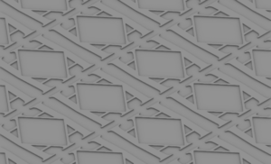
機能から形状を生成する対象として、チェッカープレートのように周期的な凹凸を有する板材を取り上げます。
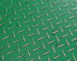
チェッカープレートの凹凸形状は滑り止めを目的していると考えられますが、このような凹凸形状は板の曲げ剛性の向上にも有効です。
このような周期的な凹凸を有する板材のマクロな曲げ特性は、連続体のシェル要素として均質化できます(以前の記事)。今回は簡単のため、直交異方性材を仮定します。また、ねじり剛性に関する成分は無視して曲げ剛性成分のみに着目します。
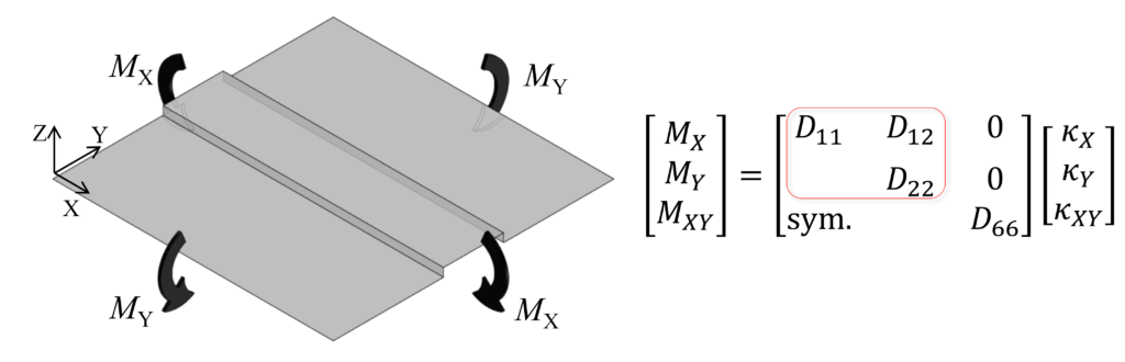
例えば、図のように凹凸がX方向に長く伸びている場合、X方向に関する曲げ剛性は高く、Y方向に関しては柔らかくなります。すなわち、曲げ剛性行列において、\(D_{11}\)成分が大きく、\(D_{22}\)成分が小さくなります。
実際の設計においては、状況に応じて「ちょうどよい特性」を有する部材が求められる場面がしばしばあります。今回は問題設定を単純化していますが、3つの曲げ特性を同時に調整することは、ある程度の専門的訓練を受けた技術者でないと容易ではないでしょう。
3. データセットの作成
生成モデルは、何もないところから作成できるわけではなく、学習するためのデータセットを準備する必要があります。
今回は、多様な形状パターンを含む学習データを作成するために、文字をもとにした凹凸形状を作成します。また、各形状に対して有限要素解析を実施し、条件ラベルに用いる曲げ剛性を算出します。

3.1 解析モデル
今回は直交異方性構造を仮定するため、文字をもとに作成された形状を1ユニット4分の1モデルとして有限要素解析を実施し、曲げ剛性を取得します。
形状作成にあたり、10×10 mmの領域に文字を配置し、それを28×28ピクセルの画像として二値化しました。画像中の文字が存在する領域をビード(凸部)とみなし、解析モデル上ではその部分を盛り上がった構造として扱います。このような角ばったビード形状は製造が困難ですが、今回の検討では解析モデル単純化のため、滑らかな曲線や高さの変化は考慮していません。

ビード高さは一律0.3 mmとし、Z方向重心を通る面を中立面と仮定します。材料条件としてはの板厚0.1 mm、ヤング率1 GPa、ポアソン比0.3を設定しました。
モデル化にはシェル要素を用い、X方向とY方向にそれぞれ曲げ変形させた際の反モーメントから曲げ剛性行列を算出します。
3.2 形状パターン
恣意的な形状選定を避け、データセットに多様性を持たせるため、ひらがなをもとにして形状を作成しました。(ひらがなの起源や形状的特徴に関しては以前の記事をご参照ください。)
使用した文字は、現代仮名遣いに用いられるひらがな46文字に加え、歴史的仮名遣いで用いられる「ゐ」および「ゑ」を含む計48文字です。フォントは游ゴシック体を採用し、スタイル(太字、斜体)や位置、スケールにバリエーションを加えることで計2304個の形状パターンを作成しました。
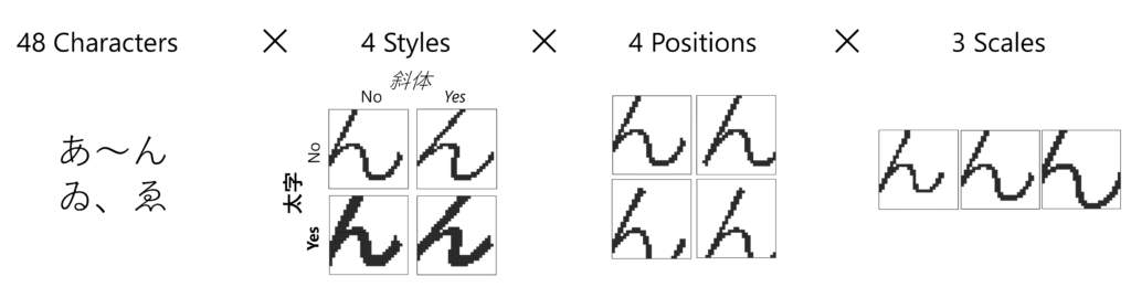
作成された各形状は28×28ピクセルの画像として保存し、生成モデルの学習に使用します。画像上では盛り上げる部分(ビード)を黒色で表現しています。
3.3 データセットの解析結果
各形状ごとの有限要素解析に要する時間は数秒程度であり、すべてのデータに対する曲げ剛性の算出は数時間で完了します。得られた曲げ剛性成分の結果を下図に示します。
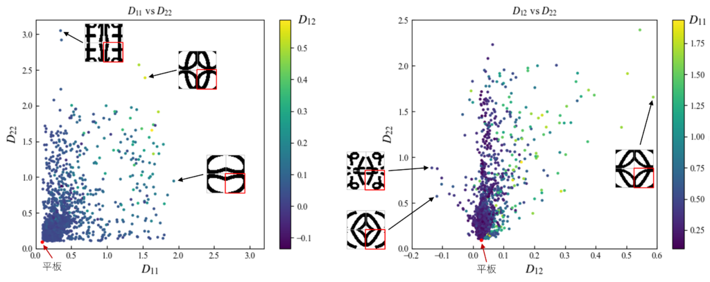
参考として、次式より計算される平板(凹凸なし)の曲げ剛性を赤点でプロットしています。

上下方向に連続する形状が多いため、全体的にy方向曲げ剛性が高い分布となっています。この内容を詳しく観察するだけでも興味深いデータとなっていますが、詳細を語るには余白が足りない本題から外れるため、今回は省略します。
3.4 データ拡張
生成モデルの学習では、学習データの量や分布の偏りがモデル性能に大きく影響します。今回のデータセットでは、文字に由来する縦方向に連続した形状が多いため、Y方向の曲げ剛性が高いサンプルが相対的に多く含まれていました。こうした偏りを緩和し、データの多様性を高めるために、データ拡張(Data Augmentation)を導入しました。
データ拡張(Data Augmentation)とは、既存のデータに対して回転や反転、スケーリングなどの処理を加えることで、データセットのバリエーションを人工的に増やす手法です。
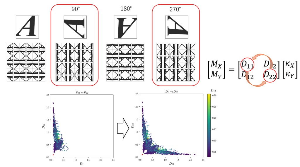
本検討では、回転操作によるデータ拡張を実施しました。
各形状に対して 180°回転を行ったものは、元の形状と同一の曲げ剛性成分を持つため、ラベルの変更なくそのまま使用可能です。一方、90°および270°回転の場合、形状の主方向が入れ替わるため、曲げ剛性行列において D₁₁成分とD₂₂成分を入れ替えることで整合の取れたラベルを付与します。
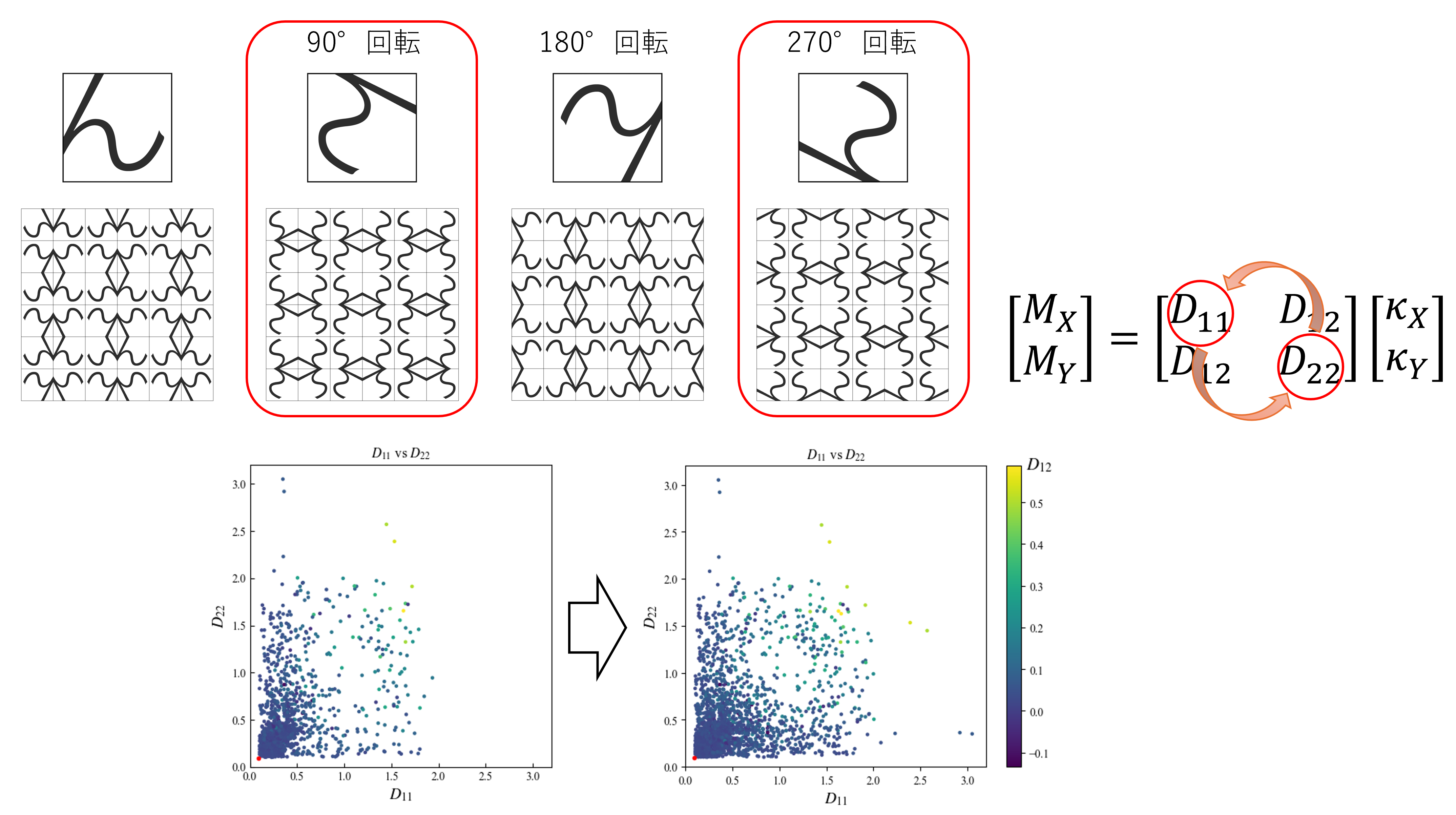
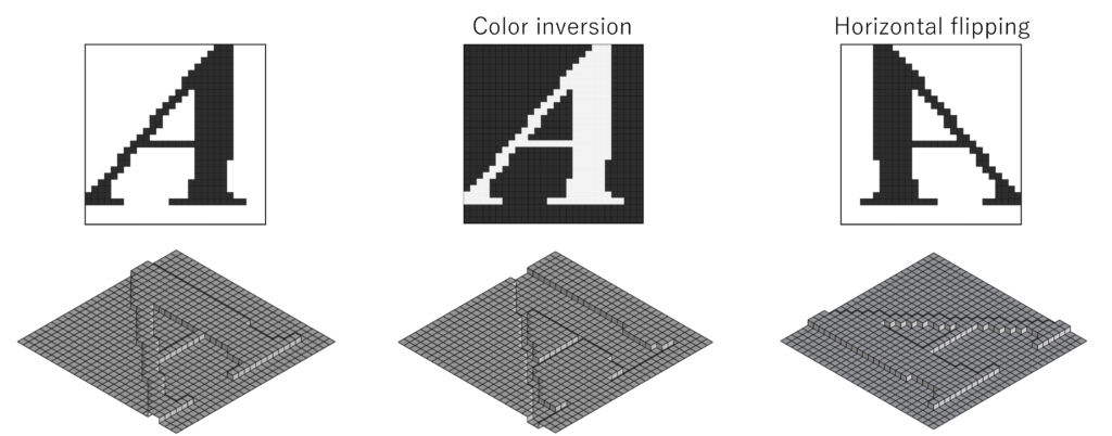
なお、白黒反転(凹凸の反転)や左右反転も同一の曲げ剛性を使用できるため、同様の拡張が可能です。
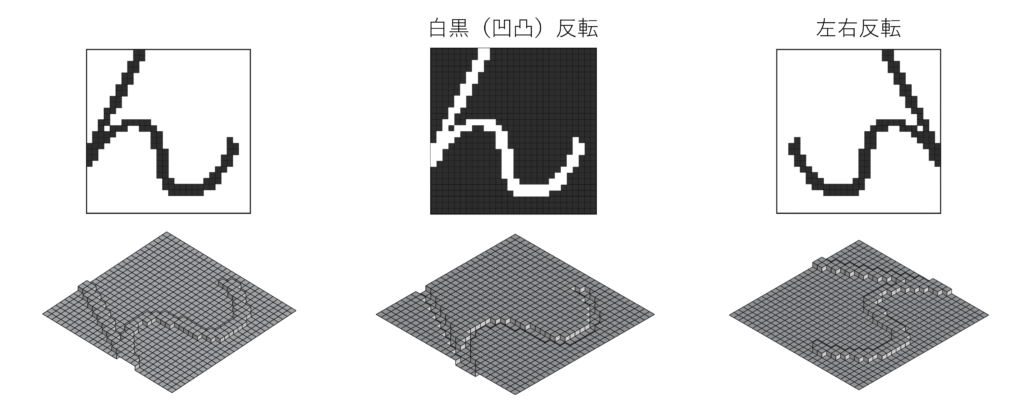
ただし、今回は出力の多様性よりも学習速度と収束性を優先し、回転操作のみを用いた拡張に限定しました。拡張により、剛性分布の偏りが改善され、データセット全体の件数は4倍に増加しています。
4. NNの構成と学習
生成モデルとして用いた条件付きGAN(cGAN)の構成と学習方法について説明します。
一般的なGANは非常に強力な生成能力を持つ手法ですが、モデルを構成しただけで、期待通りの出力が得られるとは限らず、学習そのものにも多くの課題が伴います。そのため、適切なモデル設計と綿密な試行錯誤が不可欠です。
さらに、今回の目的は指定された条件に合致する形状を生成することにあります。そのため、生成される形状が条件に忠実であること(条件忠実性)が求められます。一方で、今回の問題は1つの条件に対して複数の解が存在し得る(多義的である)という性質もあり、出力の多様性も重要な要素となります。一般に条件忠実性と多様性という相反する傾向にあるため、これらの両立にはモデル構成や学習方法に工夫が必要です。
4.1 GANにおける課題
GANには、次のような課題が存在します:
- 明示的な損失関数が存在せず、性能評価や収束判定が難しい
- 学習が不安定になりやすく、モード崩壊(Generatorが多様なサンプルを出力できなくなる)や学習不均衡(GeneratorとDiscriminatorの性能バランスが崩れ学習が停滞する)が生じる
そのため、以下のような調整が必要となります:
- GeneratorとDiscriminatorのバランスを取るように学習率を調整
- バッチサイズ、潜在空間のサイズ、ドロップアウト、活性化関数などのハイパーパラメータを調整
4.2 学習構成と工夫
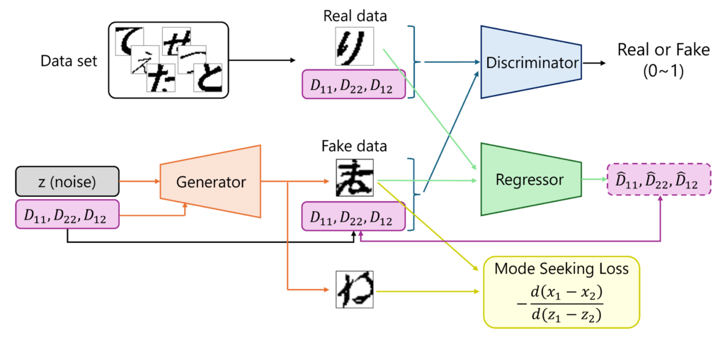
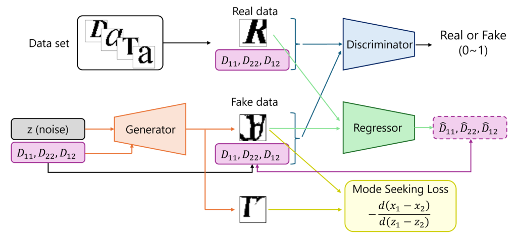
今回は、単純な生成器(Generator)と識別器(Discriminator)だけでなく、条件忠実性の向上と出力多様性の確保を目的として、いくつかの工夫を加えた構成としました。以下に、実装上の工夫、ネットワークの構成要素、および損失関数について説明します。
4.2.1 実装上の工夫
学習を安定させ、期待される出力が得られるようにするため、以下の工夫を導入しました。
- Generatorでは条件ラベルの意味付けや学習安定化のため、ラベルを中間層で注入
- 条件忠実性を保つためRegressorを導入し、生成画像から曲げ剛性を推定
- 出力多様性を保つため、入力ノイズの変化が出力差に反映されるようMode seeking損失を追加(MSGAN)
4.2.2 構成要素
本モデルは、以下の3つのネットワークから構成されます:
- 生成器(Generator):ランダムノイズ \(z\)と条件ラベル(\(D_{11}, D_{22}, D_{12}\))を入力として、画像を生成
- 識別器(Discriminator):画像と条件ラベルを受け取り、それが実データか偽データかを判定
- Regressor:生成画像から推定される曲げ剛性(\(\hat{D}_{11}, \hat{D}_{22}, \hat{D}_{12}\))を出力し、条件との整合性を確認
4.2.3 損失関数
各ネットワークの損失関数は以下のように定義しました。実画像を\(x\)、条件ラベルを\(y\)、入力ノイズを\(z\)としています。複数のサンプルをまとめたミニバッチ単位で平均を取って計算してます。
-
識別器(Discriminator)の損失:\(\text{Loss}_D = -\log D(x,y)-\log(1-D(G(z,y)),y)\)
識別器(Discriminator)は、実データ\(x\)が入力された場合は本物であると判断するように、生成データ\(G(z, y)\)に対しては偽物であると判断するように学習されます。 -
生成器(Generator)の損失:\(\text{Loss}_G=\underbrace{-\log D(G(z,y),y)}_\text{adversarial}+\underbrace{||R(G(z,y))-y||^2}_\text{regressor}+\underbrace{\text{Loss}_{MS}(G(z,y),G(z',y),z,z')}_\text{mode-seeking}\)
生成器(Generator)の損失は、識別器を騙すための項 に加え、Regressorを通じた条件忠実性の項、およびMode Seeking損失(\(\text{loss}_{MS}\))を含みます。 -
Regressorの損失:\(LossR=||R(x)-y||^2+||R(G(z,y))-y||^2\)
Regressorは、実データ\(x\)および生成データ\(G(z, y)\)のいずれに対しても、正しい曲げ剛性ラベル\(y\)を出力できるように学習されます。
ニューラルネット構成要素および学習に関して、Pytorchを用いて作成したコードの抜粋を以下に示します。必要な処理を一部省略しているため、そのままでは動作しない点をご留意ください。
class Generator(nn.Module):
    def __init__(self):
        super().__init__()

        self.noise_block = nn.Sequential(
            nn.Linear(nz, 64 * 7 * 7),
            nn.BatchNorm1d(64 * 7 * 7),
            nn.LeakyReLU(0.1),
            nn.Unflatten(1, (64, 7, 7)),  # (batch, 64, 7, 7)

            nn.ConvTranspose2d(64, 64, 4, 2, 1, bias=False),  # (batch, 64, 14, 14)
            nn.BatchNorm2d(64),
            nn.LeakyReLU(0.1),
        )

        self.label_mapper = nn.Sequential(
            nn.Linear(label_dim, 64),
            nn.BatchNorm1d(64),
            nn.LeakyReLU(0.1),
            nn.Linear(64, 64 * 14 * 14),
            nn.Tanh(),
            nn.Unflatten(1, (64, 14, 14))   # (batch, 64, 14, 14)
        )

        self.net = nn.Sequential(
            nn.ConvTranspose2d(128, 64, 4, 2, 1, bias=False),  # (batch, 64, 28, 28)
            nn.BatchNorm2d(64),
            nn.LeakyReLU(0.1),

            nn.ConvTranspose2d(64, 32, 3, 1, 1, bias=False),  # (batch, 32, 28, 28)
            nn.BatchNorm2d(32),
            nn.LeakyReLU(0.1),

            nn.ConvTranspose2d(32, 1, 3, 1, 1, bias=False),  # (batch, 1, 28, 28)
            nn.Tanh()
        )

    def forward(self, z, label):
        x = self.noise_block(z)
        label = self.label_mapper(label)
        x = torch.cat([x, label], dim=1)
        y = self.net(x)
        return y

class Discriminator(nn.Module):
    def __init__(self):
        super().__init__()
        self.net = nn.Sequential(
            nn.Conv2d(1 + label_dim, 64, 4, 2, 1),  # (batch, 64, 14, 14)
            nn.BatchNorm2d(64),
            nn.LeakyReLU(0.1),
            nn.Dropout2d(0.3),

            nn.Conv2d(64, 64, 4, 2, 1),  # (batch, 64, 7, 7)
            nn.BatchNorm2d(64),
            nn.LeakyReLU(0.1),
            nn.Dropout2d(0.3),

            nn.Conv2d(64, 128, 4, 1, 0),  # (batch, 128, 4, 4)
            nn.BatchNorm2d(128),
            nn.LeakyReLU(0.1),
            nn.Dropout2d(0.3),

            nn.Conv2d(128, 128, 3, 1, 1),  # (batch, 128, 4, 4)
            nn.BatchNorm2d(128),
            nn.LeakyReLU(0.1),

            nn.Flatten(),   # 2048
            nn.Linear(2048, 1),
            nn.Sigmoid()  # probability (0~1)
        )

    def forward(self, x, label):
        label = label.view(label.size(0), label_dim, 1, 1)  # (batch_size, label_dim, 1, 1)
        label = label.expand(label.size(0), label_dim, x.size(2), x.size(3))  # (batch_size, label_dim, img_size, img_size)

        x = torch.cat([x, label], 1)  # (batch, 1 + label_dim, img_size, img_size)
        y = self.net(x)
        return y

  class Regressor(nn.Module):
    def __init__(self):
        super().__init__()
        self.label_dim = label_dim

        self.net = nn.Sequential(
            nn.Conv2d(1, 32, kernel_size=4, stride=2, padding=1),  # (batch_size, 32, 14, 14)
            nn.BatchNorm2d(32),
            nn.LeakyReLU(0.1),

            nn.Conv2d(32, 64, kernel_size=4, stride=2, padding=1),  # (batch_size, 64, 7, 7)
            nn.BatchNorm2d(64),
            nn.LeakyReLU(0.1),

            nn.Flatten(),  # (batch_size, 3136)
            nn.Linear(64 * 7 * 7, 128),
            nn.LeakyReLU(0.1),
            nn.Linear(128, label_dim),
            nn.Tanh()
        )

    def forward(self, x):
        return self.net(x)
# --- Model instantiation ---
device = torch.device("cuda" if torch.cuda.is_available() else "cpu")
netD = Discriminator().to(device)
netG = Generator().to(device)
netR = Regressor().to(device)
# --- Loss functions ---
adv_loss_fn = nn.BCELoss() # adversarial loss
reg_loss_fn = nn.MSELoss() # regression loss
real_labels = torch.full((batch_size, 1), 0.9, device=device)
fake_labels = torch.zeros(batch_size, 1).to(device)
# --- Single-epoch training function ---
def train():
netD.train(); netG.train(); netR.train()
for real_imgs, label in dataloader:
real_imgs = real_imgs.to(device)
label = label.to(device)
# --- Discriminator update ---
optimD.zero_grad()
z = torch.randn(batch_size, nz, device=device)
with torch.no_grad():
fake_imgs = netG(z, label)
pred_fake = netD(fake_imgs, label)
pred_real = netD(real_imgs, label)
lossD = adv_loss_fn(pred_fake, fake_labels) + adv_loss_fn(pred_real, real_labels)
lossD.backward()
optimD.step()
# --- Generator update ---
optimG.zero_grad()
z = torch.randn(batch_size, nz, device=device)
fake_imgs = netG(z, label)
# Adversarial loss
pred_fake = netD(fake_imgs, label)
loss_adv = adv_loss_fn(pred_fake, real_labels)
# Regression loss
loss_reg = reg_loss_fn(netR(fake_imgs), label)
# Mode Seeking loss
z2 = torch.randn(batch_size, nz, device=device)
fake_imgs2 = netG(z2, label)
loss_ms = mode_seeking_loss(fake_imgs, fake_imgs2, z, z2)
lossG = loss_adv + lambda1 * loss_reg + lambda2 * loss_ms
lossG.backward()
optimG.step()
# --- Regressor update ---
optimR.zero_grad()
lossR = reg_loss_fn(netR(real_imgs), label) + reg_loss_fn(netR(fake_imgs), label)
lossR.backward()
optimR.step()5. 生成形状の評価
指定した条件に対して、どの程度近しい曲げ剛性を持つ形状が生成できているかを評価するため、Generatorから出力された画像をもとに凹凸形状を再構築し、有限要素解析により曲げ剛性を算出しました。
評価は、同一の条件ラベルに対して異なる5つのノイズベクトルを入力し、それぞれから生成された画像を対象に行いました。これを100 epochごとに実施し、学習の進行に伴って生成形状の曲げ剛性がどう変化するかを観察しています。
なお、学習時には各成分の条件ラベル値を次の範囲で正規化し、\([-1, 1]\)にスケーリングしています。
- \(D_{11} \in [0, 3.2]\)
- \(D_{22} \in [0, 3.2]\)
- \(D_{12} \in [-0.2, 0.6]\)
条件ラベルとして\((D_{11}, D_{22}, D_{12}) = (0.64, 0.16, 0.04)\)を指定した場合の生成形状を次に示します。
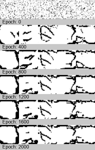
生成された形状を観察すると、文字の特徴である曲線形状が学習の進行に伴い生成されていることが分かります。また、X方向の曲げ剛性\(D_{11}\)がY方向\(D_{22}\)よりも大きい条件に対し、どちらかというとX方向に強化される形状が得られており、力学的特徴を適切に反映していることが示唆されます。さらに、入力ノイズを変化させることで異なる複数の候補形状が生成されており、多様性も確保されていることが確認できます。
また、上図の中央の画像について、生成画像を100 epochごとに有限要素解析で曲げ剛性を取得した結果を示します。
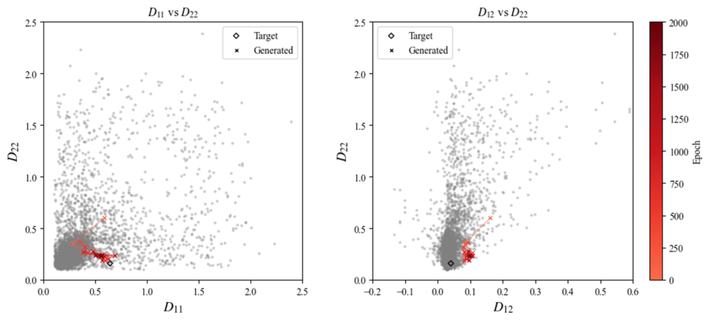
epoch数の増加に伴い、生成形状の曲げ特性が徐々に◇で示す指定条件の値に近づいていく様子が確認できます。
では、どの条件に対しても指定の曲げ剛性に近い形状を生成できるのでしょうか?
上記を含めた異なる6条件に対して生成した形状を評価しました。各条件に対して異なる5つのノイズベクトルを入力し、2000 epoch後に得られた形状の曲げ剛性を示します。
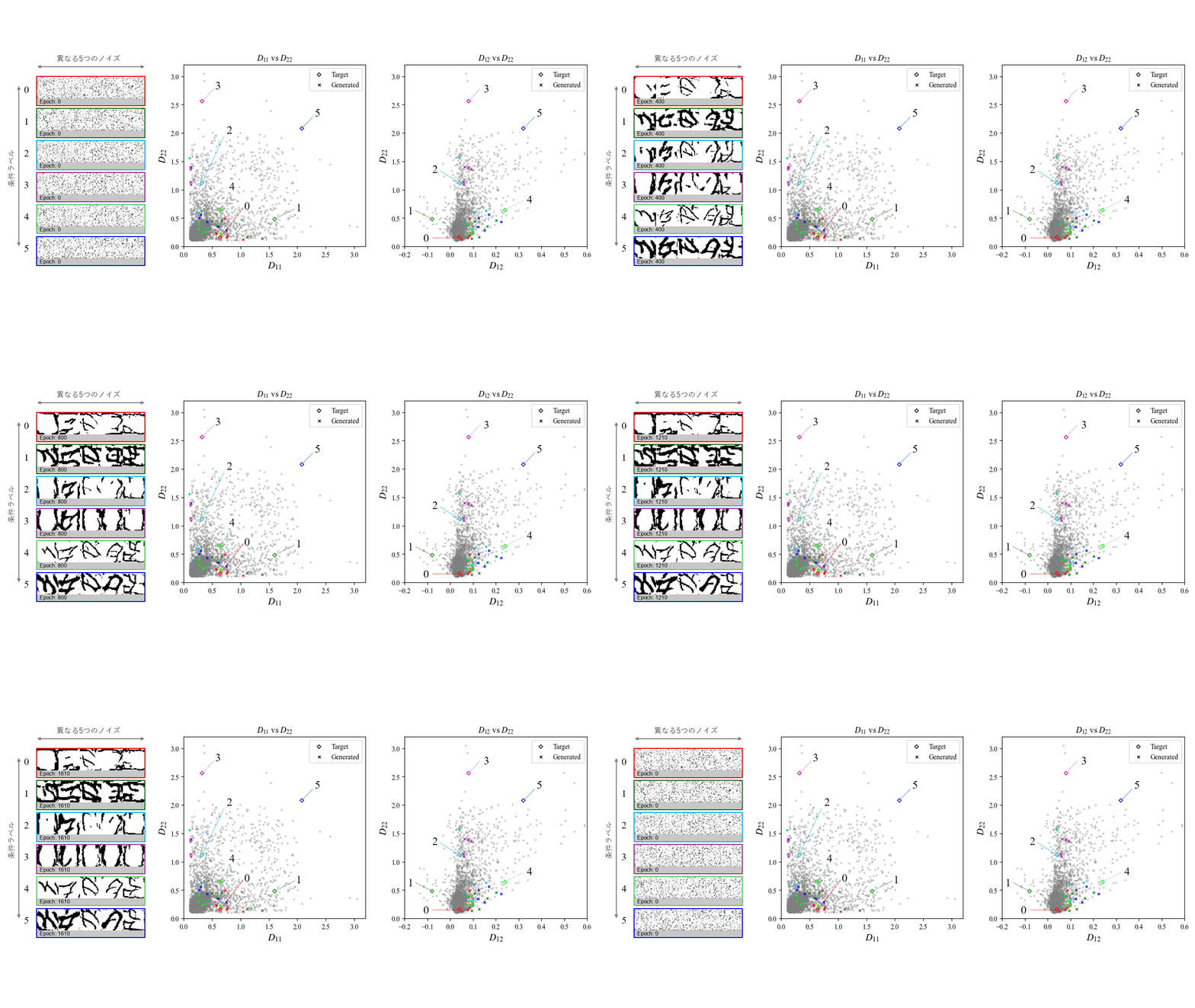
生成形状を見ると、強化する方向や剛性の大きさに応じた凹凸の大きさなど、ある程度指定条件に整合する構造形状となっていることが分かります。
一方で、色ごとに◇で示す条件ラベル値と×で示す生成結果の値を比較すると、学習データが少ない条件領域では条件忠実度が低い傾向がみられます。これは、モデルが既存データに類似した形状を生成するよう学習しているためであり、既存に存在しない条件に対応した形状を得るためには、新たなデータを加えた上で再学習を行う必要があると考えられます。
また、条件忠実度が高い条件領域でも、指定条件と生成形状との間には誤差が生じるため、現時点での実設計への応用にはなお課題が残ります。他の生成モデルの導入や、ニューラルネットワーク構造・ハイパーパラメータのより精緻な調整により、一定の改善が見込める可能性はあります。ただし、指定値により近い形状を生成するには、データセットの選別や最適化手法との併用といったアプローチが必要になると考えれます。
6. おわりに
機能条件から直接構造形状を導出する生成モデルの可能性を探るため、条件付きGAN(cGAN)を用いて検証を行いました。文字形状をもとに多様な板材凹凸形状のデータセットを作成し、曲げ剛性を指定した構造形状の生成を試みました。
結果として、曲げ剛性に応じた凹凸の方向や大きさなど、ある程度整合する形状を生成できており、単なる形状学習にとどまらず、機能を関連させた「もっともらしさ」を学習していることが示唆されました。
一方で、本手法は「形状パラメータの設定なく、誤差を許容しつつ条件を変えながら類似構造を生成する」といった場面では活用できそうなものの、実設計へ応用には次のような課題も明らかになりました:
- 専門的知識と労力が必要
データセットの準備、ネットワーク設計、ハイパーパラメータの調整などに一定の知識と試行錯誤が求められます。 - 良い構造の生成には、良い構造が必要
既存データに類似した形状を生成するため、未知条件領域では条件忠実性が低下します。
また、本手法は最適化ではないため「求める機能になりそうな形状」であり「望ましい条件を満たす形状」や「機能の実現に必要な形状」を得ることができません。
適切な構造形状を生成するためには、最適化結果を学習させる等、良質な形状をデータセットとする必要があります。
今回の検討を通じて、我々の最適化ベースの形状設計を超えるような「機能条件を入力するだけで適切な形状を自動生成する」生成モデルの実現には長い道のりがあることが分かりました。
形状設計に対する深層学習の適用可能性については継続的に検討しつつ、より高品質な形状生成を目指して取り組んでいきたいと思います。
英語版ではひらがなではなくアルファベットをデータセットに利用しています。データセットによる違いなど興味がある方は英語版と比較してみてください。(右下のENから変更できます。)
参考文献
本稿を執筆するにあたり、以下の文献を参考にしました。
[1] Xiaoyang Zheng et al. Controllable inverse design of auxetic metamaterials using deep learning. Materials & Design. 2021, 221, 110178
[2] Jan-Hendrik Bastek et al. Inverse design of nonlinear mechanical metamaterials via video denoising diffusion models, Nature Machine Intelligence. 2023, 5, 1446-1475
0. Introduction
Deep learning (DL)–based generative techniques have advanced remarkably, making it increasingly common to automatically generate text or images from simple prompts. These generative models can produce plausible outputs based on training data, without the need for explicitly defined rules or parameter settings.
In contrast, our company's design workflows involve deriving structural geometries from functional requirements by applying a variety of optimization methods. Each method has its strengths and weaknesses, and considerable effort is required in problem formulation, parameter tuning, and method integration—often through extensive trial and error.
A DL-based generative model that directly produces structural geometries from specified conditions could eliminate much of this trial-and-error and dramatically improve design efficiency. The key question, then, is whether such a model—one that accepts functional specifications as input and outputs appropriate geometries—can be realized in the structural design domain.
1. Generative Models
A generative model learns the distribution of training data and produces new “plausible” samples that resemble the training data.
There are many types of deep neural network–based generative models. In this work, I adopt the Generative Adversarial Network (GAN), as it was the quickest for me to understand and implement.
A GAN consists of two networks—a Generator and a Discriminator—that are trained in opposition. Through this adversarial training, the Generator becomes capable of producing images that closely resemble the training set. The main advantages are that it can generate outputs with sharp, well-defined edges and do so at high speed.
In a standard GAN, the generated images depend entirely on random noise, so there is no way to control the output.
To address this, we employ a Conditional GAN (cGAN). By feeding the condition label into both the Generator and the Discriminator, cGAN enables the generation of outputs that conform to the specified condition. This approach can be applied to tasks such as generating structural geometries that meet specific functional requirements.
In this article, I omit a detailed description of generative models. For a more precise and comprehensive explanation, please refer to specialized books or academic literature.
2. Design Target
As the subject for functional-to-geometric generation, we focus on a plate with periodic corrugations—such as a checker plate.
The corrugation pattern of a checker plate is primarily designed for anti-slip purposes, but it also serves to enhance the plate’s bending stiffness.
The macroscopic bending behavior of a periodically corrugated plate can be homogenized and modeled as a continuous shell element (see our previous article). For simplicity, we here assume an orthotropic material and ignore torsional stiffness, focusing exclusively on the bending stiffness components.
For example, as illustrated in the figure, if the corrugations extend predominantly in the x-direction, the plate exhibits higher bending stiffness about the X-axis and lower stiffness about the Y-axis. In other words, in the bending stiffness matrix, the \(D_{11}\) component is large while the \(D_{22}\) component is small.
In practical design, there are often situations where a member must have just the right combination of stiffness properties. Although we simplify the problem setting here, simultaneously tuning three bending stiffness parameters is not an easy task unless performed by a technician with specialized training.
3. Dataset Preparation
A generative model cannot be created from scratch—it requires a suitable dataset for training.
To build a dataset with diverse shape patterns, we generate corrugated geometries based on different characters. We then perform finite element analysis on each geometry to compute its bending stiffness, which serves as the condition label for training.
3.1 Analysis Model
For this study, we assume an orthotropic structure and perform finite element analysis (FEA) on a quarter-unit model of each character-based geometry to extract its bending stiffness.
To generate the geometries, each character is placed within a 10 × 10 mm square and then binarized into a 28 × 28 pixel image. Regions corresponding to the character are interpreted as beads (raised portions). Although such sharp-edged beads would be difficult to manufacture in reality, we deliberately omit any smoothing of curves or height variations here to keep the analysis model simple.

The bead height is uniformly set to 0.3 mm, and and the plane passing through the center of mass in the Z direction is assumed to be the neutral plane. Material properties are defined as a plate thickness of 0.1 mm, Young’s modulus of 1 GPa, and Poisson’s ratio of 0.3. Shell elements are used for modeling, and the bending stiffness matrix is computed from the reaction moments obtained when the model is bent about the X- and Y-axes.
3.2 Geometry Patterns
To avoid arbitrary shape selection and ensure dataset diversity, we generated geometries based on the English alphabet.
We used all 52 English alphabet characters (A–Z and a–z). Using the Times New Roman font, we applied variations in font style (regular, bold, italic, and bold–italic) and in placement (position and scale) to generate 2,496 distinct shape patterns.
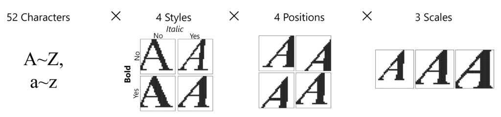
Each generated shape is saved as a 28 × 28-pixel image for training the generative model. In these images, the raised regions (beads) are depicted in black.
3.3 Analysis Results of Dataset
Finite element analysis (FEA) for each individual shape takes only a few seconds, allowing the computation of bending stiffness across the entire dataset to complete in a matter of hours. The resulting bending stiffness components are plotted in the figure below.
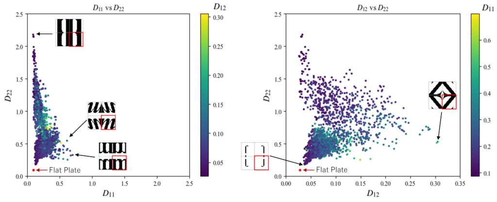
As a reference, we also plot the bending stiffness of a flat plate (without corrugations), calculated by the following formula, as red dots.
Because many of our patterns feature elements aligned along the vertical axis, the overall distribution shows higher bending stiffness in the Y-direction. Although this dataset alone would merit a detailed analysis, which this margin is too narrow to contain, doing so would fall outside the scope of this article and is therefore omitted.
3.4 Data Augmentation
In training generative models, both the quantity of training data and the distributional bias can significantly affect model performance. In the present dataset, many of the shapes derived from characters exhibit vertical continuity, resulting in a relatively large number of samples with high bending stiffness in the y-direction. To mitigate this bias and enhance the diversity of the training data, we introduced data augmentation.
Data augmentation is a technique that artificially increases dataset variation by applying transformations—such as rotations, flips, and scaling—to existing samples.
In this study, we performed augmentation using rotations:
- 180° rotation: The rotated shape has identical bending-stiffness components, so it can be used with its original labels unchanged.
- 90° and 270° rotations: These rotations swap the shape’s principal directions, so we exchange the \(D_{11}\) and \(D_{22}\) components in the bending-stiffness matrix to keep the labels consistent.
Note that color inversion (inverting bead and recess) and horizontal flipping also preserve the same bending‐stiffness values and could be applied in the same way. However, we prioritized training speed and convergence stability over maximizing output diversity, so we limited augmentation to rotations only.
As a result, the total dataset size was quadrupled.
4. NN Architecture and Training
In this section, we describe the architecture and training methodology of our Conditional GAN (cGAN)–based generative model. While standard GANs are known for their powerful generation capabilities, constructing the model alone does not definitely lead to satisfactory outputs; training presents its own set of challenges that require careful design and extensive experimentation.
Moreover, our goal is to generate shapes that faithfully satisfy specified functional conditions. This condition fidelity must be balanced against the inherently multi-modal nature of the problem, in which multiple valid solutions may exist for a single condition. Since fidelity and output diversity often exhibit conflicting tendencies, achieving both requires thoughtful architectural choices and training strategies.
4.1 Challenges in Training GANs
Generative Adversarial Networks (GANs) are known to suffer from several challenges:
- The absence of an explicit loss function in GANs complicates the evaluation of performance and the assessment of convergence.
- Training tends to be unstable, and issues such as mode collapse (where the generator fails to produce diverse outputs) and training imbalance (where the Generator and Discriminator diverge in performance, leading to stalled) often occur.
To mitigate these problems, the following adjustments are typically required:
- Fine-tuning the learning rates to maintain a balance between the Generator and Discriminator.
- Carefully selecting and tuning hyperparameters such as batch size, latent space dimensionality, dropout rate, and activation functions.
4.2 Training Architecture and Design Strategies
In this study, we adopted a training architecture that goes beyond a simple Generator–Discriminator setup. To improve conditional fidelity and ensure output diversity, we introduced several key design strategies. This section outlines the implementation techniques, network components, and loss functions used in our model.
4.2.1 Implementation Design
To stabilize training and obtain the expected outputs, we introduced the following implementation strategies:
-
Intermediate label injection in the Generator:
To give meaning to the conditional labels and help stabilize learning, the labels are injected into the intermediate layers of the Generator. -
Introduction of a Regressor for condition fidelity:
To maintain fidelity to the specified conditions, a Regressor is added to predict bending stiffness from the generated images. -
Addition of Mode Seeking Loss (MSGAN):
To ensure diversity in the output, a mode seeking loss is introduced so that changes in input noise result in differences in the generated output.
4.2.2 Components
The model consists of the following three networks:
-
Generator :
Takes random noise \(z\) and condition labels \((D_{11}, D_{22}, D_{12})\) as input and generates an image. -
Discriminator :
Takes an image and condition labels as input and determines whether the input is real (from the dataset) or fake (generated). -
Regressor :
Predicts the bending stiffness\((\hat{D}_{11}, \hat{D}_{22}, \hat{D}_{12})\) from the generated image and checks its consistency with the input condition.
4.2.3 Loss Functions
The loss functions for each network are defined as follows. Here, \(x\) denotes a real image, \(y\) denotes the condition label, and \(z\) denotes the input noise. The losses are computed as averages over mini-batches of multiple samples.
-
Discriminator loss : \(\text{Loss}_D = -\log D(x,y)-\log(1-D(G(z,y),y))\)
The Discriminator is trained to output a high probability when a real data sample is input, and a low probability when a generated (fake) sample is input. -
Generator loss : \(\text{Loss}_G=\underbrace{-\log D(G(z,y),y)}_\text{adversarial}+\underbrace{||R(G(z,y))-y||^2}_\text{regressor}+\underbrace{\text{Loss}_{MS}(G(z,y),G(z',y),z,z')}_\text{mode-seeking}\)
The Generator’s loss consists of the adversarial term (to fool the Discriminator), a regression term via the Regressor to ensure consistency with the condition, and the Mode Seeking Loss \(\text{Loss}_{\text{MS}}\) to encourage output diversity.
-
Regressor loss : \(LossR=||R(x)-y||^2+||R(G(z,y))-y||^2\)
The Regressor is trained to output the correct bending stiffness labels \(y\) for both real data x and generated data \(G(z, y)\).
Below is an excerpt of the PyTorch-based code used to construct and train the neural networks. Please note that some auxiliary processes have been omitted for brevity, and the code may not run as-is.
class Generator(nn.Module):
    def __init__(self):
        super().__init__()

        self.noise_block = nn.Sequential(
            nn.Linear(nz, 64 * 7 * 7),
            nn.BatchNorm1d(64 * 7 * 7),
            nn.LeakyReLU(0.1),
            nn.Unflatten(1, (64, 7, 7)),  # (batch, 64, 7, 7)

            nn.ConvTranspose2d(64, 64, 4, 2, 1, bias=False),  # (batch, 64, 14, 14)
            nn.BatchNorm2d(64),
            nn.LeakyReLU(0.1),
        )

        self.label_mapper = nn.Sequential(
            nn.Linear(label_dim, 64),
            nn.BatchNorm1d(64),
            nn.LeakyReLU(0.1),
            nn.Linear(64, 64 * 14 * 14),
            nn.Tanh(),
            nn.Unflatten(1, (64, 14, 14))   # (batch, 64, 14, 14)
        )

        self.net = nn.Sequential(
            nn.ConvTranspose2d(128, 64, 4, 2, 1, bias=False),  # (batch, 64, 28, 28)
            nn.BatchNorm2d(64),
            nn.LeakyReLU(0.1),

            nn.ConvTranspose2d(64, 32, 3, 1, 1, bias=False),  # (batch, 32, 28, 28)
            nn.BatchNorm2d(32),
            nn.LeakyReLU(0.1),

            nn.ConvTranspose2d(32, 1, 3, 1, 1, bias=False),  # (batch, 1, 28, 28)
            nn.Tanh()
        )

    def forward(self, z, label):
        x = self.noise_block(z)
        label = self.label_mapper(label)
        x = torch.cat([x, label], dim=1)
        y = self.net(x)
        return y

class Discriminator(nn.Module):
    def __init__(self):
        super().__init__()
        self.net = nn.Sequential(
            nn.Conv2d(1 + label_dim, 64, 4, 2, 1),  # (batch, 64, 14, 14)
            nn.BatchNorm2d(64),
            nn.LeakyReLU(0.1),
            nn.Dropout2d(0.3),

            nn.Conv2d(64, 64, 4, 2, 1),  # (batch, 64, 7, 7)
            nn.BatchNorm2d(64),
            nn.LeakyReLU(0.1),
            nn.Dropout2d(0.3),

            nn.Conv2d(64, 128, 4, 1, 0),  # (batch, 128, 4, 4)
            nn.BatchNorm2d(128),
            nn.LeakyReLU(0.1),
            nn.Dropout2d(0.3),

            nn.Conv2d(128, 128, 3, 1, 1),  # (batch, 128, 4, 4)
            nn.BatchNorm2d(128),
            nn.LeakyReLU(0.1),

            nn.Flatten(),   # 2048
            nn.Linear(2048, 1),
            nn.Sigmoid()  # probability (0~1)
        )

    def forward(self, x, label):
        label = label.view(label.size(0), label_dim, 1, 1)  # (batch_size, label_dim, 1, 1)
        label = label.expand(label.size(0), label_dim, x.size(2), x.size(3))  # (batch_size, label_dim, img_size, img_size)

        x = torch.cat([x, label], 1)  # (batch, 1 + label_dim, img_size, img_size)
        y = self.net(x)
        return y

  class Regressor(nn.Module):
    def __init__(self):
        super().__init__()
        self.label_dim = label_dim

        self.net = nn.Sequential(
            nn.Conv2d(1, 32, kernel_size=4, stride=2, padding=1),  # (batch_size, 32, 14, 14)
            nn.BatchNorm2d(32),
            nn.LeakyReLU(0.1),

            nn.Conv2d(32, 64, kernel_size=4, stride=2, padding=1),  # (batch_size, 64, 7, 7)
            nn.BatchNorm2d(64),
            nn.LeakyReLU(0.1),

            nn.Flatten(),  # (batch_size, 3136)
            nn.Linear(64 * 7 * 7, 128),
            nn.LeakyReLU(0.1),
            nn.Linear(128, label_dim),
            nn.Tanh()
        )

    def forward(self, x):
        return self.net(x)
# --- Model instantiation ---
device = torch.device("cuda" if torch.cuda.is_available() else "cpu")
netD = Discriminator().to(device)
netG = Generator().to(device)
netR = Regressor().to(device)
# --- Loss functions ---
adv_loss_fn = nn.BCELoss() # adversarial loss
reg_loss_fn = nn.MSELoss() # regression loss
real_labels = torch.full((batch_size, 1), 0.9, device=device)
fake_labels = torch.zeros(batch_size, 1).to(device)
# --- Single-epoch training function ---
def train():
netD.train(); netG.train(); netR.train()
for real_imgs, label in dataloader:
real_imgs = real_imgs.to(device)
label = label.to(device)
# --- Discriminator update ---
optimD.zero_grad()
z = torch.randn(batch_size, nz, device=device)
with torch.no_grad():
fake_imgs = netG(z, label)
pred_fake = netD(fake_imgs, label)
pred_real = netD(real_imgs, label)
lossD = adv_loss_fn(pred_fake, fake_labels) + adv_loss_fn(pred_real, real_labels)
lossD.backward()
optimD.step()
# --- Generator update ---
optimG.zero_grad()
z = torch.randn(batch_size, nz, device=device)
fake_imgs = netG(z, label)
# Adversarial loss
pred_fake = netD(fake_imgs, label)
loss_adv = adv_loss_fn(pred_fake, real_labels)
# Regression loss
loss_reg = reg_loss_fn(netR(fake_imgs), label)
# Mode Seeking loss
z2 = torch.randn(batch_size, nz, device=device)
fake_imgs2 = netG(z2, label)
loss_ms = mode_seeking_loss(fake_imgs, fake_imgs2, z, z2)
lossG = loss_adv + lambda1 * loss_reg + lambda2 * loss_ms
lossG.backward()
optimG.step()
# --- Regressor update ---
optimR.zero_grad()
lossR = reg_loss_fn(netR(real_imgs), label) + reg_loss_fn(netR(fake_imgs), label)
lossR.backward()
optimR.step()5. Evaluation of Generated Geometries
To evaluate how closely the generated geometries match the specified bending stiffness conditions, we reconstructed the surface profile from the images output by the Generator and computed the bending stiffness using finite element analysis.
For each condition label, five different noise vectors were input, and the corresponding generated images were evaluated. This process was repeated every 100 epochs to observe how the bending stiffness of the generated shapes evolved over the course of training.
Note that during training, the values of each component of the condition labels were normalized to the range of \([-1, 1]\).
- \(D_{11} \in [0, 2.5]\)
- \(D_{22} \in [0, 2.5]\)
- \(D_{12} \in [0, 0.350]\)
The following shows the generated shapes when the condition label \((D_{11}, D_{22}, D_{12}) = (0.5, 0.25, 0.0875)\) is specified.
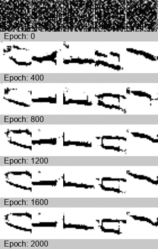
Observing the generated shapes, we can see that the curved features characteristic of letters gradually emerge as training progresses. Moreover, given that the bending stiffness in the X-direction \(D_{11}\) is larger than that in the Y-direction \(D_{22}\), the generated shapes tend to be reinforced in the X-direction, suggesting that the model appropriately reflects the mechanical characteristics.
In addition, by changing the input noise, multiple distinct shape candidates are generated, confirming that the model also ensures diversity in its outputs.
The results of the finite element analysis conducted every 100 epochs on the leftmost image above are shown below, where the bending stiffness values were calculated for each generated image.
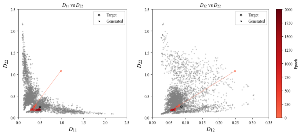
As the number of training epochs increases, the bending characteristics of the generated shapes gradually approach the target values indicated by the diamond symbol (◇).
But can the model generate shapes with bending stiffness close to the specified conditions for any given input?
To explore this, we evaluated the shapes generated for 6 different conditions, including the one mentioned above. For each condition, 5 different noise vectors were input, and the bending stiffness values of the resulting shapes after 2000 training epochs are shown.
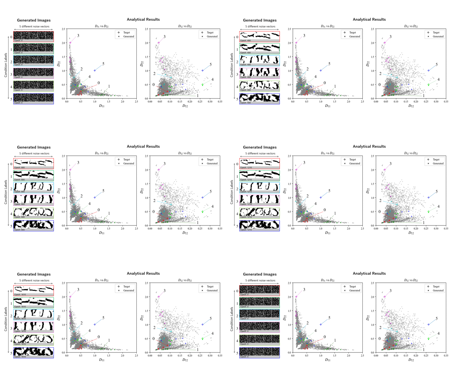
When examining the generated shapes, we can see that the overall structure generally aligns with the specified conditions—for example, the direction of reinforcement and the prominence of the corrugation correspond to the magnitude and directionality of the target stiffness.
On the other hand, when comparing the target values (marked with diamonds ◇) and the generated results (marked with crosses ×) by color, we observe that in regions where training data is sparse, the model tends to show lower condition fidelity. This is because the model is trained to generate shapes similar to the existing data, and to produce shapes that correspond to conditions not covered in the training set, it will likely require additional data and retraining.
Moreover, even in condition regions with high fidelity, discrepancies between the specified conditions and the generated geometries remain, indicating that further challenges must be addressed before the method can be applied in practical design. Incorporating alternative generative models or refining the neural network architecture and hyperparameters may offer some improvements. However, to generate shapes that more closely match the target conditions, it will likely be necessary to adopt approaches such as selective dataset curation or combining with optimization-based techniques.
6. Conclusion
To explore the potential of generative models that derive structural geometries directly from functional requirements, we conducted an investigation using a Conditional GAN (cGAN). A diverse dataset of corrugated plate geometries was constructed based on letter shapes, and we attempted to generate structural forms conditioned on specified bending stiffness values.
As a result, the model was able to generate geometries that showed a degree of consistency with the target stiffness—such as the direction and magnitude of corrugation—suggesting that it learned not only shapes but also a form of "plausibility" related to mechanical function.
At the same time, while this approach may prove useful in scenarios where similar structures need to be generated without explicitly setting shape parameters, allowing for some margin of error, several challenges remain before it can be applied in real-world structural design:
-
Requires expertise and effort
Preparing the dataset, designing the network, and tuning hyperparameters all demand domain knowledge and iterative experimentation. -
Good structures require good data
Because the model learns to generate shapes similar to existing data, condition fidelity tends to degrade in regions not well covered by the dataset.
Moreover, since this method is not an optimization process, it produces shapes that might satisfy the desired function, but not necessarily those that do or must. In order to generate appropriate geometries, the dataset needs to consist of high-quality, functionally effective structures—such as those obtained from optimization results.
We have come to recognize the approach presented here is not yet sufficient to realize a generative model that can automatically produce appropriate geometries solely from functional input—something that could surpass our current optimization-based design methods.
We intend to continue exploring the applicability of deep learning to geometry design, striving toward higher-quality structural generation.
In the Japanese version of this article, hiragana characters are used for the dataset instead of the alphabet. If you are interested in comparing the differences between datasets, please take a look at the Japanese version. (You can switch to it using the "JP" button in the bottom-right corner.)
References
The following works were referenced during the writing of this article:
