
1質点系の動的な性能について
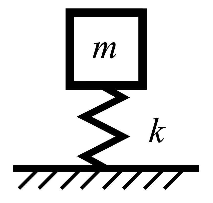
以下のような質量 \(m\)、バネ剛性 \(k\) の非減衰の1質点のバネマス系について考えます。
自由振動
質点が自由振動している状態での変位および力の関係は以下のように表すことができます。
\(\begin{align}
m \ddot{x} + kx = 0 \tag{1-1} \\
\ddot{x} + \omega_n^2 x = 0 \tag{1-2} \\
\omega_n^2 = \frac{k}{m} \tag{1-3}
\end{align}\)
上記微分方程式の一般解は以下のようになり、オイラーの公式よりサイン波で表される単振動になります。
\(x=Ae^{i\omega_n t + \delta}\)
\(A\)は最大振幅、\(\delta\) は位相差で初期値に依存する値です。一般解からわかるように \(\omega_n\) は \(2\pi\) 秒内で何回振動するかを表す量で固有円振動数と呼ばれます。
固有円振動数 \(\omega_n\) は、固有周期 \(T\)、固有周波数 \(f_n\) とは次の関係があります。
\(f_n = \frac{1}{T} = \frac{\omega_n}{2 \pi} = \frac{1}{2 \pi} \sqrt{\frac{k}{m}}
\tag{1-4}\)
式(1-4)より質量が一定の場合は、剛性の平方根に比例して固有周波数は高くなること、つまり剛性が高くなる(固くなるほど)固有周波数が高くなることがわかります。
強制振動
次に以下のような強制振動の問題において固有周波数が変化すると応答がどのように変化するかを考えます。
式(1-1) で扱っていた自由振動の問題に対して、円振動数 \(\omega\)、振幅 \(|F_0|\) の強制振動 \(F_0 = |F_0| e^{i \omega t}\) が与えられた状況を考えます
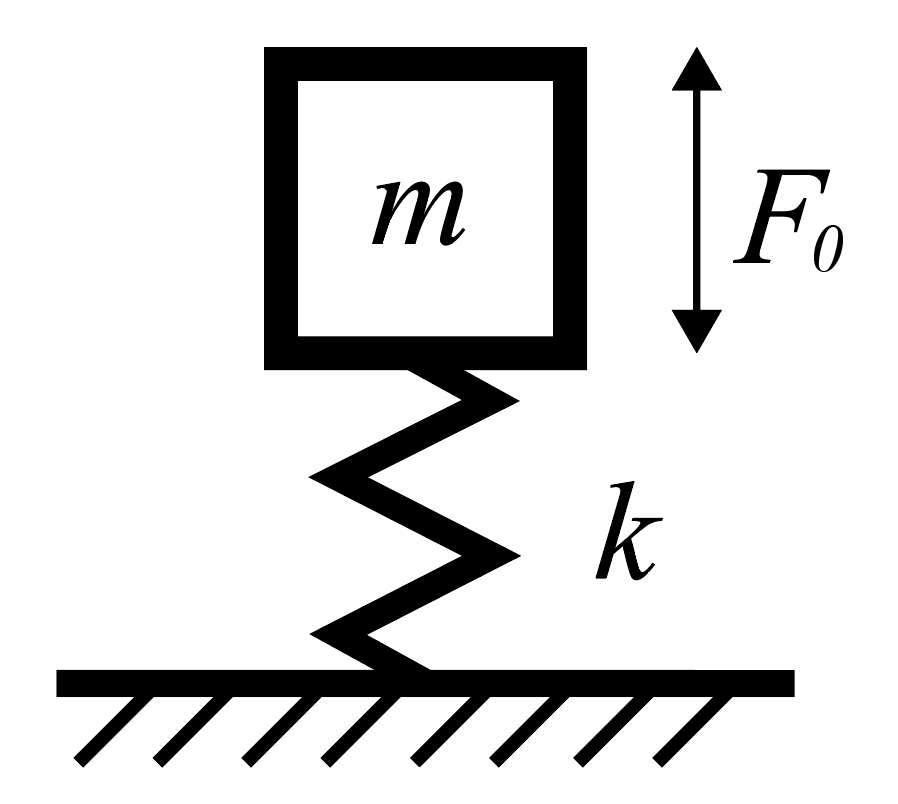
質点周りの力の釣り合いより、加振された質点の運動方程式は以下のようになります。
\(\ddot{x} + \omega_n^2 x = F_0
\tag{1-5}\)
一方で、このバネを介して振動が伝わり、支持点側で発生する反力 \(F\) は、バネが変形することによって発生するため式(1-5)の2項目から、支持点まわりの力の釣り合いを考えると次のようになります。
\(\omega_n^2 x = F
\tag{1-6}\)
以上より振動源から支持部への振動の伝達率 \(T_r\) は 式(1-5)、式(1-6) の比をとって以下のようになります。
\(\begin{align}
T_r &= \left|\frac{F}{F_0} \right|
= \left|\frac{\omega_n^2 x}{\ddot{x} + \omega_n^2 x} \right|
= \left|\frac{1}{1 + \frac{1}{\omega_n^2} \frac{\ddot{x}}{x}} \right| \\
&= \left|\frac{1}{1 + \frac{-\omega^2}{\omega_n^2}} \right|
= \left|\frac{1}{1 - u^2} \right|
\tag{1-7}
\end{align}\)
\(u\) は加振周波数と1質点系の固有周波数の比(\(u=\frac{\omega}{\omega_n} = \frac{f}{f_n}\))、\(x\) は式(1-5) の形式の微分方程式の一般解 \(x = A e^{i \omega t}\) を使用して解いています。
式(1-7) をグラフ化すると以下になります。
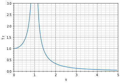
これらより次のことがわかります。
- \(u = 1\) のとき、振動が大きく増幅して伝達される(共振現象)
- \(u\) が \(\sqrt{2}\) 以下の範囲では常に振動が増幅される
- \(u\) が \(\sqrt{2}\) を超えたときはじめて振動伝達率 \(Tr\) の値が 1 を下回り防振効果を発揮する
つまり防振したい場合は、周波数の比を \(\sqrt{2}\) 以上にする必要があります。
具体的な防振設計例
100Hz で加振される 1kg の装置から発生する振動の伝達を \(\frac{1}{8}\) となるように防振したい場合、周波数比 \(u=3\) となり目標の固有周波数は式(1-7) より以下になります。
\(3 = \frac{100}{f_n}, \quad
\tag{1-8}
f_n \fallingdotseq 33 [\rm{Hz}]\)
式(1-4) よりこのときのバネ剛性 \(k\) は次のようになります。
\(\frac{100}{3} = \frac{1}{2 \pi} \sqrt{\frac{k}{1}}, \quad
k = \left( \frac{200}{3} \pi \right)^2 \fallingdotseq 43900 [\textrm{N/m}] = 43.9 [\textrm{N/mm}]
\tag{1-9}\)
実際の防振設計では、既製品で上記で求まった性能とぴったり一致する部材があることは少ないので近い値の部材をカタログから探すなどします。
各防振部材メーカーはウェブやカタログなどに選定フローがあり細かく計算しなくともどういった防振部材を選べばいいか書いてあったり表やグラフで求められる場合が多いです。
質量と周波数の関係
複数の質量と加振周波数の組み合わせでの防振について計算した結果を以下の表にまとめました。
| 質量 \(m\) [kg] | 加振周波数 \(F_0\) [Hz] | 伝達率が 1/8 となる(\(u = 3\)) となる固有周波数 \(F_n\) [Hz] | バネ剛性 \(k\) [N/mm] |
|---|---|---|---|
| 1 | 100 | 33 | 43.9 |
| 0.1 | 100 | 33 | 4.39 |
| 0.01 | 100 | 33 | 0.439 |
| 1 | 10 | 3.3 | 0.439 |
| 0.1 | 10 | 3.3 | 0.0439 |
| 0.01 | 10 | 3.3 | 0.00439 |
| 1 | 1 | 0.33 | 0.00439 |
| 0.1 | 1 | 0.33 | 0.000439 |
| 0.01 | 1 | 0.33 | 0.0000439 |
このように、軽いものをより低い加振周波数でも防振するためには、より低い剛性のバネが求められることがわかります。
このバネ剛性で具体的にはどのような形状の部材があるかは、例えばモノタロウさんやミスミさんなどで、バネ剛性の値から部品を検索することができるので、興味がある方は調べてみてください。
上記表にある 1kg の質点を 10Hz で加振したときに防振するために必要な剛性 0.439N/mm の部材の一例として単純なコイルばねの以下のような既製品の部材がありました。
| 材質 | 自由高(mm) | 外径(Φmm) | 線径(Φmm) | ばね定数 (N/mm) |
|---|---|---|---|---|
| SUS304 | 40 | 11 | 0.8 | 0.44 |
1質点系の静的な性能について
これまで計算してきた振動に対する問題(動的な問題)に対して、以下のように重力加速度 \(g\) がかかるのみの部材の静的な状態について考えます。
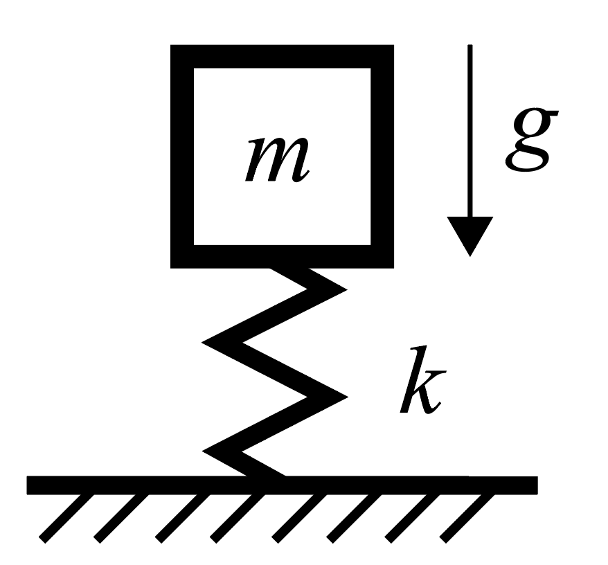
自重でのたわみ \(\delta\) は力のつり合いより下式になります。
\(\delta = \frac{m g}{k}
\tag{2-1}\)
式(2-1)より、質量が一定の場合は剛性が大きくなるほどたわみが小さくなることがわかります。
1kg のものを 10Hz の加振に対して防振に必要だと求めた上記表のコイルばねの静的な変位を考えます。
\(\delta = \frac{1 \times 9.8}{0.44} = 22.2 \textrm{mm}
\tag{2-2}\)
静的たわみ量が 22.2mm となり、バネの自然長 40mm の半分以上を静的な荷重で変形してしまっています。
防振用途での使用する際はこの変位から強制振動時の変形が加わるので、このように静的な状態で大きく変形してしまっている場合は、強制振動時の変形で底付きが発生し(バネが40mm変形してバネが接触し)防振効果を失い、衝突による大きな荷重が防振対象に掛かる可能性があります。
上記例では 1kg、10Hz の防振ですが、より低い周波数の防振の場合を想定し 1kg、1Hz の防振を考えるとバネ剛性 \(k\) は1/100 になります。このときの変形量は \(22.2 \times 100 = 2220\textrm{[mm]} = 2.22\textrm{[m]}\) と非現実的な値となり、これまで紹介してきた手法では防振が困難な結果です。
剛性-質量-周波数のトレードオフについて
これまで示してきた動的な特性と静的な特性をまとめると、以下のトレードオフがあることがわかります。
- 剛性が小
- 1次固有周波数が低くなるため、より低周波数から防振することができる
- 静的たわみが大きくなり、防振対象物を設置しただけで過大な変形が発生し底付きする可能性がある。
- 剛性が大
- 1次固有周波数が高い周波数になるため、防振が難しくなる
- 静的たわみが小さくなり、重量物でも安定して支えることができる。
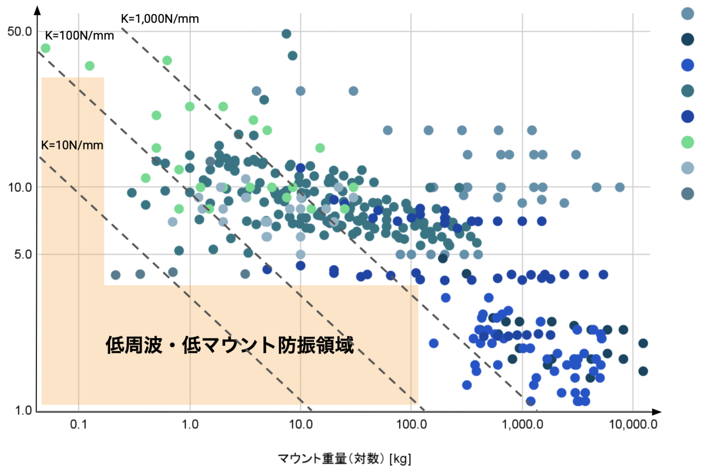
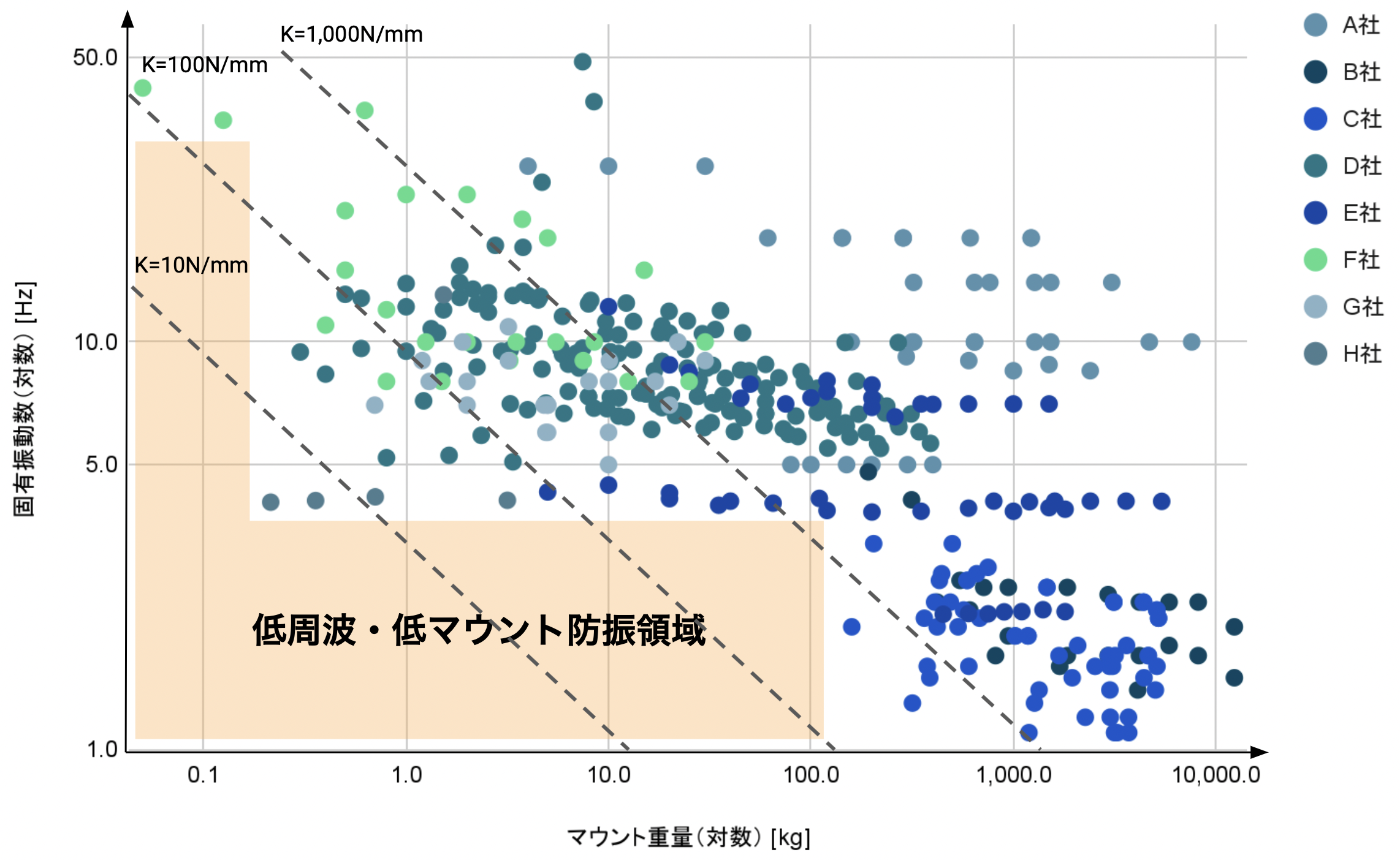
弊社で以前に既製品の防振部材を調査した結果が以下です。
低い周波数での防振を行おうとすると静的な変位が過大になってしまうこのトレードオフがあるため、低周波数の範囲で既製品の防振部材が市販されていないことがわかります。
低周波数の防振を実現しているグラフの右下の点の部材は、空気バネ方式と呼ばれる特殊なバネ剛性を持つ部材で防振を行っています。
まとめ
一般的な動剛性と静剛性、及びそれらから求まる防振のトレードオフについて紹介しました。
次の記事では、最後に紹介したトレードオフを突破できる可能性のある構造メタマテリアルの一つの QZS と呼ばれる構造の具体的な内容について紹介します。
About the dynamic performance of 1 mass-spring model
Consider the following undamped 1 mass-spring model with mass \(m\) and spring stiffness \(k\).
Free vibration
The relationship between displacement and force with the point mass in free vibration can be expressed as follows
\(\begin{align}
m \ddot{x} + kx = 0 \tag{1-1} \\
\ddot{x} + \omega_n^2 x = 0 \tag{1-2} \\
\omega_n^2 = \frac{k}{m} \tag{1-3}
\end{align}\)
\(\omega_n\) is called the natural circular frequency, which has the following relationship with the natural period \(T\) and natural frequency \(f_n\).
\(f_n = \frac{1}{T} = \frac{\omega_n}{2 \pi} = \frac{1}{2 \pi} \sqrt{\frac{k}{m}}
\tag{1-4}\)
Equation (1-4) shows that for constant mass, the natural frequency increases in proportion to the square root of the stiffness, i.e., the higher the stiffness, the higher the natural frequency.
Forced Vibration
Next, consider how the response changes as the natural frequency changes in the following forced vibration problem. For the free vibration problem treated in Equation (1-1), consider the situation where a forced vibration \(F_0\) at an circular frequency of \(\omega\) is given.
The equation of motion of a vibrated point mass from the balance of forces is as follows
\(\ddot{x} + \omega_n^2 x = Fe^{i \omega t} = F_0
\tag{1-5}\)
On the other hand, the vibration is transmitted through this spring, and the reaction force \(F\) generated at the support point side is generated by the term affected by the spring in equation (1-5), which is
\(\omega_n^2 x = F
\tag{1-6}\)
From the above, the transmission coefficient of vibration from the vibration source to the support, \(T_r\), is obtained by taking the ratio of Equations (1-5) and (1-6) as follows
\(\begin{align}
T_r &= \left|\frac{F}{F_0} \right|
= \left|\frac{\omega_n^2 x}{\ddot{x} + \omega_n^2 x} \right|
= \left|\frac{1}{1 + \frac{1}{\omega_n^2} \frac{\ddot{x}}{x}} \right| \\
&= \left|\frac{1}{1 + \frac{-\omega^2}{\omega_n^2}} \right|
= \left|\frac{1}{1 - u^2} \right|
\tag{1-7}
\end{align}\)
\(u\) is the ratio of the excitation frequency to the natural frequency of the 1 mass-spring model (\(u=\frac{\omega}{\omega_n} = \frac{f}{f_n}\)), and \(x\) is solved using the general solution \(x = A e^{i \omega t}\) of the differential equation of the form (1-5).
Equation (1-7) can be graphed as follows
From these we can see the following
- When \(u = 1\), vibrations are transmitted with great amplification (resonance phenomenon)
- Vibrations are always amplified in the range \(u\) less than \(\sqrt{2}\).
- Only when \(u\) exceeds \(\sqrt{2}\), the value of vibration transmission coefficient \(Tr\) falls below 1 and vibration isolation is achieved.
In other words, if you want to isolate vibration, the ratio of frequencies must be greater than \(\sqrt{2}\).
Specific vibration isolation design examples
If we wish to isolate the transmission of vibration generated by a 1 kg device vibrated at 100 Hz so that \(\frac{1}{8}\), the frequency ratio \(u=3\) and the target natural frequency is the following from equation (1-7).
\(3 = \frac{100}{f_n}, \quad
\tag{1-6}
f_n \fallingdotseq 33 [\rm{Hz}]\)
From equation (1-4), the spring stiffness \(k\) in this case is
\(\frac{100}{3} = \frac{1}{2 \pi} \sqrt{\frac{k}{1}}, \quad
k = \left( \frac{200}{3} \pi \right)^2 \fallingdotseq 43900 [\textrm{N/m}] = 43.9 [\textrm{N/mm}]
\tag{1-7}\)
In actual vibration isolation design, it is rare to find off-the-shelf components that exactly match the performance obtained above, so it is necessary to search for components with similar values in catalogs.
In many cases, vibration isolation component manufacturers provide a selection flow on their websites or in their catalogs, which describes what type of vibration isolation component to select without detailed calculations, or provide tables and graphs to help you find the right component.
Mass vs. frequency
The following table summarizes the results of calculations for vibration isolation for several combinations of mass and excitation frequency.
| Mass \(m\) [kg] | Excitation frequency \(F_0\) [Hz] | The transfer coefficient becomes 1/8 (\(u = 3\)) Natural frequency \(F_n\) [Hz] | Spring stiffness \(k\) [N/mm] |
|---|---|---|---|
| 1 | 100 | 33 | 43.9 |
| 0.1 | 100 | 33 | 4.39 |
| 0.01 | 100 | 33 | 0.439 |
| 1 | 10 | 3.3 | 0.439 |
| 0.1 | 10 | 3.3 | 0.0439 |
| 0.01 | 10 | 3.3 | 0.00439 |
| 1 | 1 | 0.33 | 0.00439 |
| 0.1 | 1 | 0.33 | 0.000439 |
| 0.01 | 1 | 0.33 | 0.0000439 |
Thus, we can see that a lower stiffness spring is required to isolate lighter objects even at lower excitation frequencies.
If you are interested in finding out what specific shapes of components are available with this spring stiffness, you can search for components by spring stiffness value at, for example, Monotaro or MISUMI, and so on.。
As an example of a member with the stiffness of 0.439 N/mm required to isolate vibration when a 1 kg mass point in the above table is vibrated at 10 Hz, the following ready-made member of a simple coil spring was found.
| Material | Natural height(mm) | Diameter(Φmm) | wire diameter(Φmm) | spring stiffness (N/mm) |
|---|---|---|---|---|
| SUS304 | 40 | 11 | 0.8 | 0.44 |
Static performance of 1 mass-spring model
In contrast to the problems so far calculated for vibration (dynamic problems), the following is considered for the static state of a member subjected only to gravitational acceleration \(g\).
The deflection under its own weight \(\delta\) is given by the following equation from the balance of forces.
\(\delta = \frac{m g}{k}
\tag{2-1}\)
Equation (2-1) shows that for a constant mass, the greater the stiffness, the smaller the deflection.
Consider the static displacement of the coil spring in the table above, which is determined to be necessary for vibration isolation of a 1 kg spring against 10 Hz excitation.
\(\delta = \frac{1 \times 9.8}{0.44} = 22.2 \textrm{mm}
\tag{2-2}\)
The static deflection is 22.2mm, which means that more than half of the spring's natural length of 40mm has been deformed by the static load.
When the spring is used for vibration isolation, deformation during forced vibration is added from this displacement, so if the spring is greatly deformed in the static state, it may bottom out due to deformation during forced vibration (the spring is deformed 40 mm and the spring makes contact), losing its vibration isolation effect, and a large load from a collision may be applied to the object to be isolated. The object may be subjected to a large load due to a collision.
In the above example, the vibration isolation is 1 kg at 10 Hz, but assuming a lower frequency vibration isolation, the spring stiffness \(k\) is 1/100 of 1 kg at 1 Hz. The amount of deformation in this case is \(22.2 \times 100 = 2220\textrm{[mm]} = 2.22\textrm{[m]}\), an unrealistic value that makes it difficult to achieve vibration isolation with the methods introduced so far.
On the stiffness-mass-frequency tradeoff
Summarizing the dynamic and static characteristics I have shown so far, we can see that there is a tradeoff between
- Less stiffness
- Lower first-order natural frequencies allow vibration isolation from lower frequencies
- Static deflection is increased and excessive deformation may occur and bottom out just by installing the vibration isolating object.
- Greater stiffness
- Vibration isolation becomes more difficult due to the higher first-order natural frequencies
- Static deflection is reduced and even heavy objects can be supported stably.
The following is the result of a previous survey of off-the-shelf anti-vibration components.
Because of this trade-off, we find that there are no off-the-shelf vibration isolation components commercially available in the low-frequency range.
The member at the lower right point of the graph that achieves low-frequency vibration isolation is a member with special spring stiffness, called an air-spring system.
Summary
This article introduced dynamic and static stiffness and the tradeoffs for vibration isolation that can be obtained from them.
In the next article, I will introduce the specifics of one of the structural metamaterials, called QZS, that may be able to break through the tradeoffs introduced in the last section.
