
はじめに
エンジニアの岡です。本年もよろしくお願いします。
弊社では幾何学と力学が密接に関連した設計を日々行っていますが、本記事では(すでに1月も下旬になってしまいましたが)お正月のしめ縄飾りの形状を力学的に考えてみたいと思います。
しめ縄飾りの形
お正月に玄関などに飾られるしめ縄にはさまざまな形状がありますが、稲藁から直線状の縄を作っておき、曲げて部分的に固定することで輪などの形にしているものをよく見ます。水引についても、和紙をよった直線状の材料を曲げることで作られています。
これはしなやかな棒の両端に変位境界条件を与えている状態とみなせます。なお、しめ縄も水引も物によっては材料の非線形性や重力の影響が大きくなっているものもありますが、本記事では材料の弾性範囲で曲げ変形が支配的になっている状況を考えます。
-scaled.jpg)
エラスティカ曲線
このようなしなやかな棒曲げによって生じる曲線はエラスティカ曲線と呼ばれ、17世紀ごろから物理学者たちの研究対象になってきました。身の回りの例として、自転車のブレーキ等のワイヤー、ギターの弦、電源ケーブルなどが、おおよそエラスティカ曲線の振る舞いをします。
機械系の材料力学で一般的に学ぶ梁の曲げは、たわみ角が微小な場合の理論でした。エラスティカ曲線でも「中立軸に垂直な断面はが変形後も平面を保ち中立軸に垂直である」という前提は同じですが、たわみ角が微小でないと仮定している点が異なります。
エラスティカ曲線が満たすべき条件はエネルギ最小化問題として記述することができます。曲げエネルギーは曲率 \(\kappa\) の2乗に比例することから、次の式の弾性エネルギ \(E[\kappa (s)]\) 最小にするような \(\kappa (s)\) を求めることができれば、曲線の形状を知ることができます。なお \(s\) は弧長パラメータ、 \(l\) は棒の全長です。
\(E[κ(s)] = ∫_0^l κ(s)^2 ds\)
曲線の形は材料物性や断面形状に依らず、境界条件と全長のみで決定されます。
上式から得られる微分方程式の解析解は18世紀にオイラーが示していますが、この記事では便利なツールを使って数値的に解くことにします。
Kangarooを使った数値解析
今回は3D CADのRhino/Grasshopper環境で使用できるKangaroo2と呼ばれるプラグインを使用します。Kangaroo2では、様々な物理的な条件(Goal)に基づくエネルギー最小化問題を解くことなどにより形状をモデリングすることができます。強度計算など部材に作用する応力を知りたい場合には不向きですが、今回のしめ縄形状のように、材料や断面係数に関係なく決まる棒の変形形状を知りたい場合には適しています。
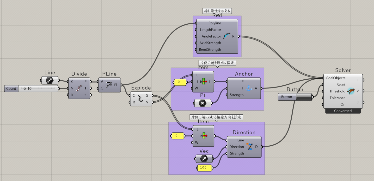
今回使用するメインの機能はRodコンポーネントです。変形させたい棒を細かな線分に分割してRodコンポーネントに入力すると、隣り合う線分同士の成す角の変化量に比例したモーメントが生じます。これにより棒状物体の曲げ剛性を表現することができます。

境界条件はAnhcorコンポーネントおよびDirectionコンポーネントで付与します。Anhcorコンポーネントは固定したい節点と、固定したい場所の座標を入力することで、両者が一致するような剛性を設定できます。Directionコンポーネントは、梁要素とベクトルを入力すると、両者が平行になるように剛性が生じます。これらの剛性は上記Rodの剛性よりも十分大きくしておく必要があります。(下の図では、片方の端の境界条件のみ与えています。)
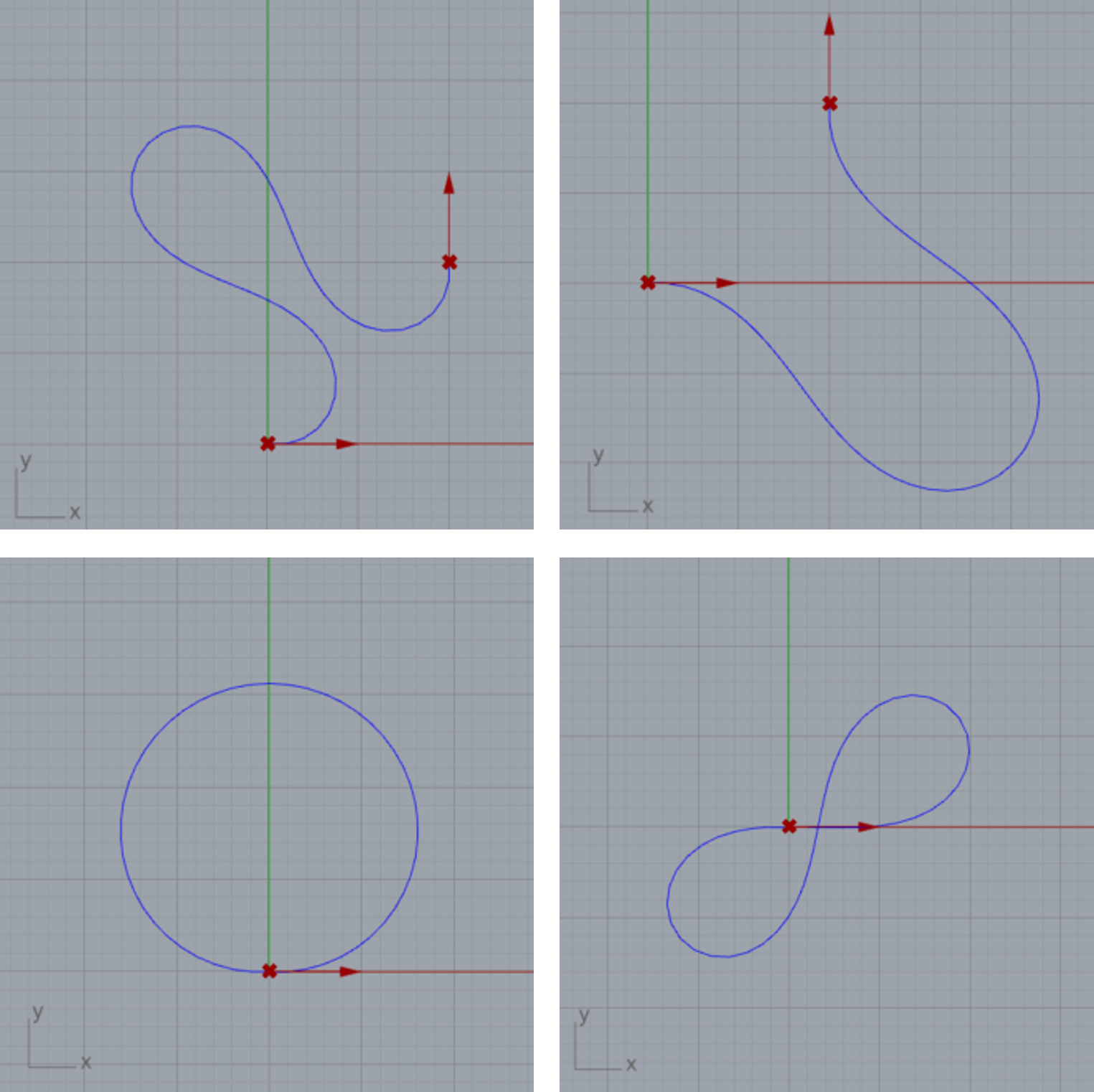
以下は2種類の境界条件でを与えた場合の変形形状の例です。×印が固定位置、矢印が固定位置の棒の角度を示しています。上2つと、下2つはそれぞれ同一の境界条件ですが、左右でことなる安定状態となっておいり、前回記事で紹介されていた双安定構造とみることもできます。
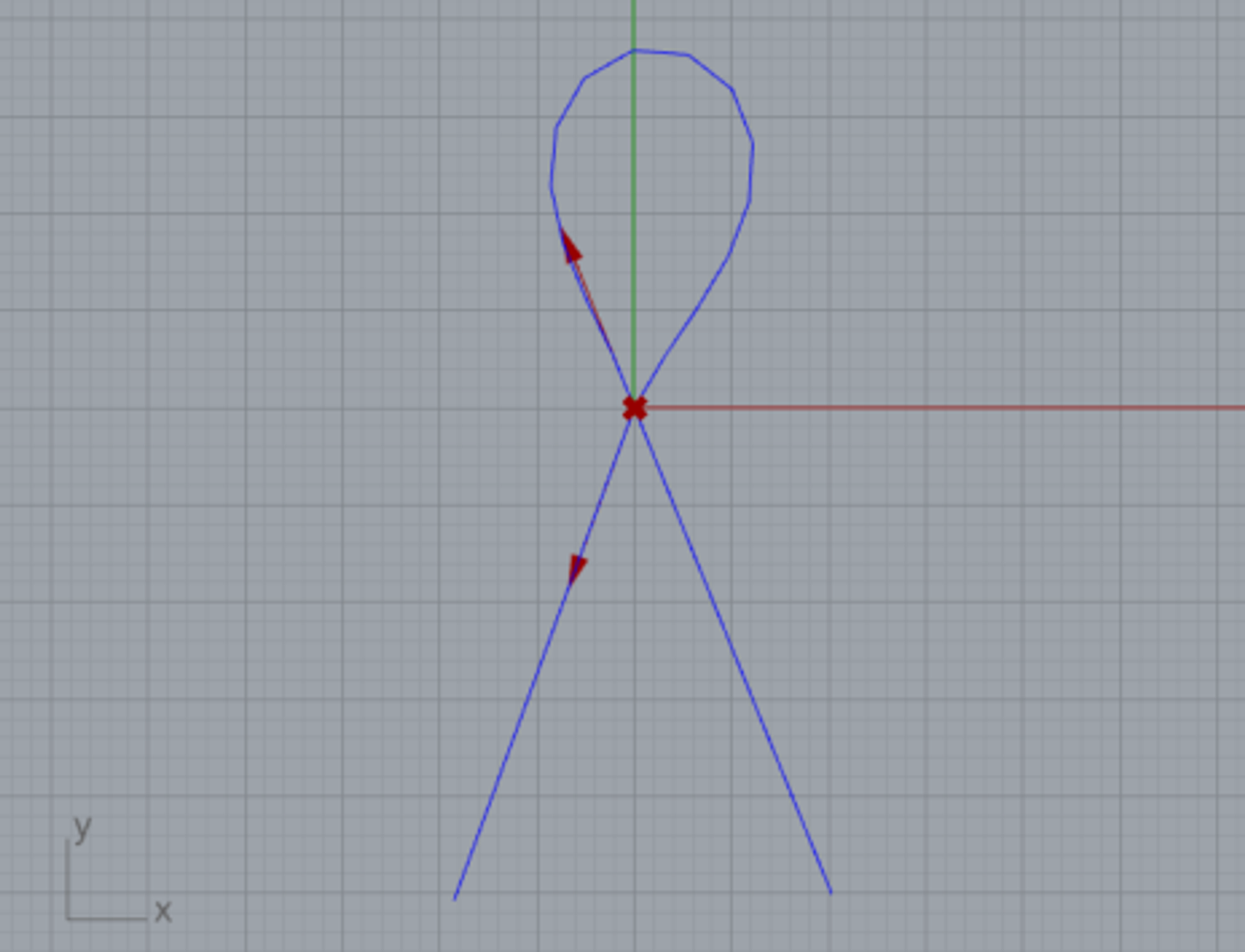
しめ縄形状をシミュレートしてみましょう。冒頭の写真をイメージして、直線上の棒(稲藁の縄)を曲げて輪を作り、固定します。上記例とは異なり、境界条件を与える点を直線の両端ではなく途中にすることで、固定部から端は直線となります。
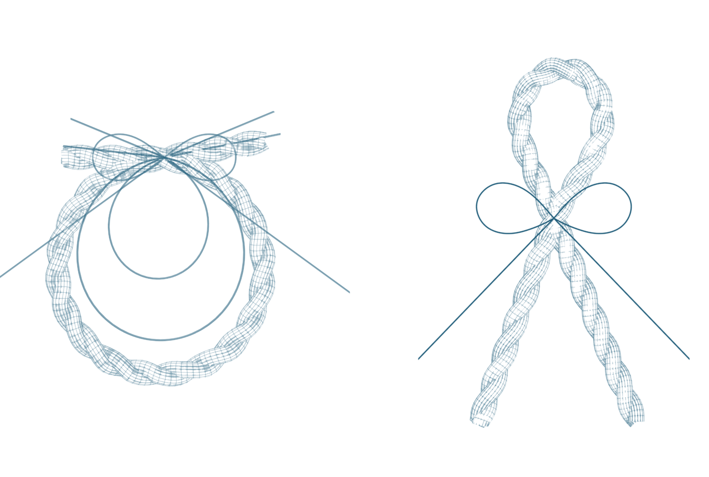
これだけでは味気ないので、水引部分を追加し、さらに縄部分をモデリングしてみると以下のようになりました。CGとしてはかなり雑ですが、ある程度写真のしめ縄に近い形状になったのではないでしょうか。
水引部分に関しては、現物よりも曲率がやや小さくなっているように見受けられます。実際の水引では曲率が大きい部分が弾性的でない変形をしたり、クリープすることでより曲率が大きくなっているものと推測されます。
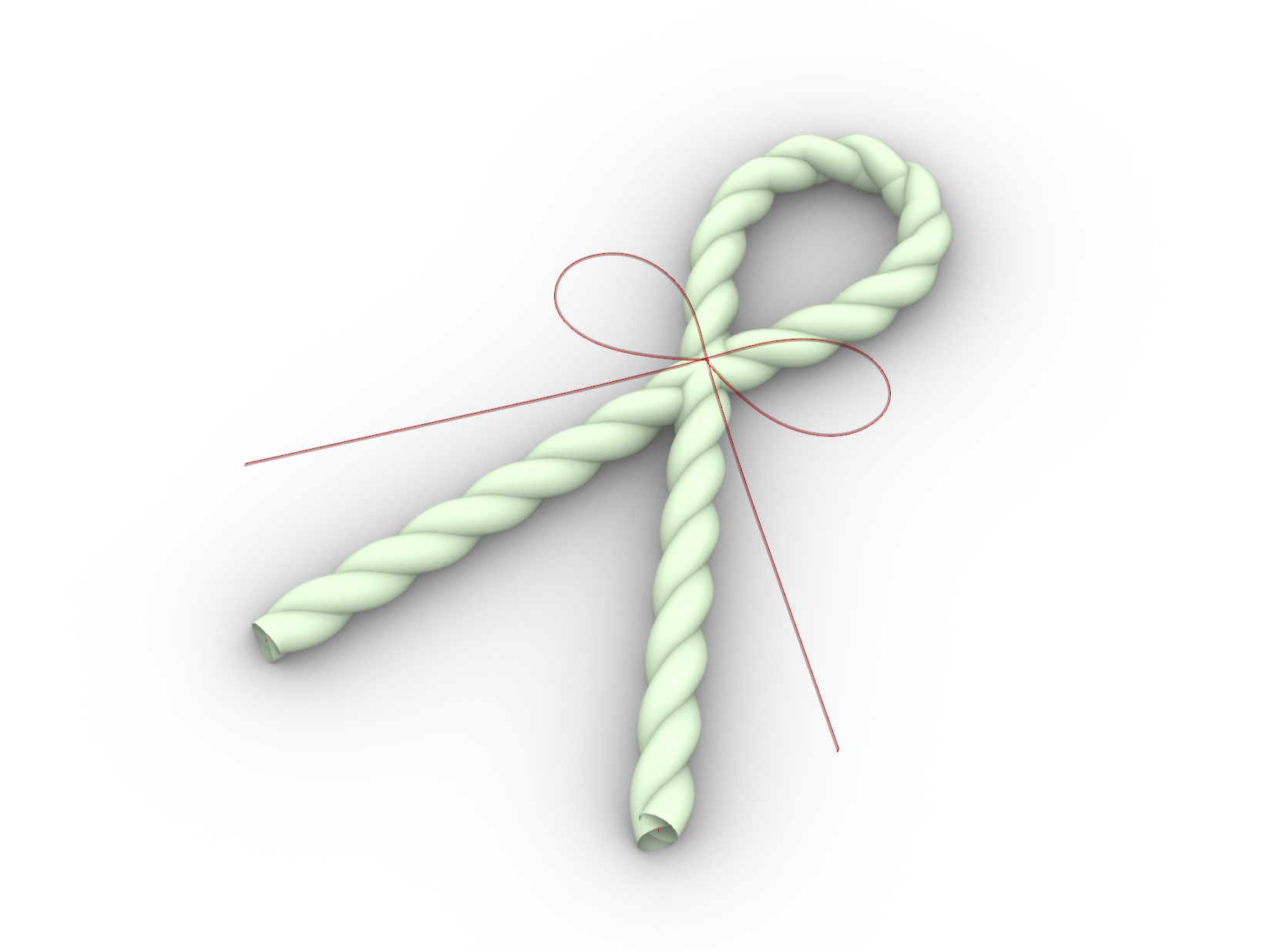
冒頭の写真の輪形状のものについてもモデリングしてみると以下のようになりました。

さいごに
本記事ではエラスティカ曲線のシミュレーションによりしめ縄の形状の再現を試みました。理想的な弾性曲げ以外の影響もあるので正確とは言えませんが、しめ縄の形状の種類を、エラスティカ曲線の境界条件のバリエーションと捉えることはできるのではないでしょうか。
お正月は過ぎてしまいましたが、しめ縄以外にも同様の性質を示す物体はいろいろあるので、みなさんも身の回りのエラスティカ曲線を探してみてはいかがでしょうか。
参考文献
[1] Levien, R. L. (2009). From Spiral to Spline: Optimal Techniques in
Interactive Curve Design. University of California, Berkeley. https://levien.com/phd/thesis.pdf
[2] Daniel Piker. (2019/1/19). How does Kangaroo solver work?. Rinoceros Forums. https://discourse.mcneel.com/t/how-does-kangaroo-solver-work/92075
Introduction
In our company, we are involved in design work where geometry and mechanics are closely intertwined. Although it's already late January, in this article, I would like to mechanically analyze the shape of the New Year's Shimenawa decorations.
The Shape of Shimenawa Decorations
During the New Year, various shapes of Shimenawa are commonly seen decorating entrances. These are typically made from straw ropes that are straight initially and then bent and partially fixed to form shapes like loops. Similarly, Mizuhiki (decorative Japanese cords) are also made by bending materials like twisted paper that are initially straight.
This can be considered as a state where displacement boundary conditions are given to both ends of a flexible rod. Note that depending on the material, the non-linearity of the material or the effect of gravity can be significant for both Shimenawa and Mizuhiki. However, in this article, we will consider situations where bending deformation is dominant within the elastic range of the material.
The Elastica Curve
Such curves formed by bending flexible rods are known as Elastica curves and have been the subject of study by physicists since around the 17th century. Examples in our daily life like the wires of bicycle brakes, guitar strings, and power cables, approximately behave according to the Elastica curve.
The bending of beams commonly studied in the material mechanics of mechanical systems is based on the theory where the angle of deflection is small. While Elastica curves also assume the same premise that "sections perpendicular to the neutral axis remain plane and perpendicular to the neutral axis after deformation", they differ in that they do not assume the angle of deflection to be small.
The conditions that Elastica curves must satisfy can be described as an energy minimization problem. Since the bending energy is proportional to the square of the curvature \(\kappa\), we can determine the shape of the curve by finding the curvature \(\kappa(s)\) that minimizes the elastic energy \(E[\kappa(s)]\). Here, \(s\) is the arc length parameter, and \(l\) is the total length of the rod.
\(E[κ(s)] = ∫_0^l κ(s)^2 ds\)
The shape of the curve is determined solely by the boundary conditions and the total length, regardless of the material properties or cross-sectional shape.
Euler presented an analytical solution to the differential equation derived from the above equation in the 18th century. However, in this article, we will solve it numerically using a convenient tool.
Numerical Analysis with Kangaroo
This time, we use a plugin called Kangaroo2, available in the 3D CAD Rhino/Grasshopper environment. With Kangaroo2, you can model shapes by solving energy minimization problems based on various physical conditions (Goals). It's not suitable for understanding the stresses acting on members, such as in strength calculations, but it's appropriate for understanding the deformation shapes of rods determined regardless of material or sectional coefficients, like the shape of the Shimenawa in this case.
The main feature we'll use this time is the Rod component. When you input a rod you want to deform into the Rod component after dividing it into fine line segments, a moment proportional to the change in the angle formed by adjacent line segments occurs. This allows you to represent the bending stiffness of rod-like objects.
Boundary conditions are applied using the Anchor and Direction components. The Anchor component allows you to set rigidity such that the node you want to fix and the coordinates of the place you want to fix it coincide by inputting both. The Direction component generates rigidity that makes the beam element and vector parallel when inputted. The rigidity of these should be significantly larger than that of the aforementioned Rod.
Below are examples of deformation shapes given two types of boundary conditions. The 'x' marks indicate fixed positions, and the arrows show the angle of the rod at the fixed position. The top two and the bottom two have the same boundary conditions, respectively, but are in different stable states, which can also be seen as bistable structures introduced in the previous article.
Let's simulate the shape of the Shimenawa. Imagining the first photo, we bend a rod (straw rope) in a straight line to form a loop and fix it. Unlike the above examples, by setting the boundary conditions at points along the line other than the ends, the parts from the fixed point to the ends remain straight.
To add a bit more flair, we add the Mizuhiki part and model the rope part, resulting in the following appearance. Although it's quite rough as a CG, it's somewhat close to the shape of the actual Shimenawa in the photo.
For the Mizuhiki part, the curvature appears to be slightly smaller than the actual object. It's presumed that in the actual Mizuhiki, parts with larger curvature undergo non-elastic deformation or creep, resulting in larger curvature.
When we also model the ring-shaped object in the first photo, we get the following.
Conclusion
In this article, we attempted to reproduce the shape of the Shimenawa through simulation of Elastica curves. While it's not entirely accurate due to the influence of factors other than ideal elastic bending, it may be possible to understand the variety of Shimenawa shapes as variations in the boundary conditions of Elastica curves.
Although the New Year has passed, there are various objects around us that exhibit similar properties to Shimenawa, so why not look for Elastica curves in your surroundings?
References
[1] Levien, R. L. (2009). From Spiral to Spline: Optimal Techniques in
Interactive Curve Design. University of California, Berkeley. https://levien.com/phd/thesis.pdf
[2] Daniel Piker. (2019/1/19). How does Kangaroo solver work?. Rinoceros Forums. https://discourse.mcneel.com/t/how-does-kangaroo-solver-work/92075
