
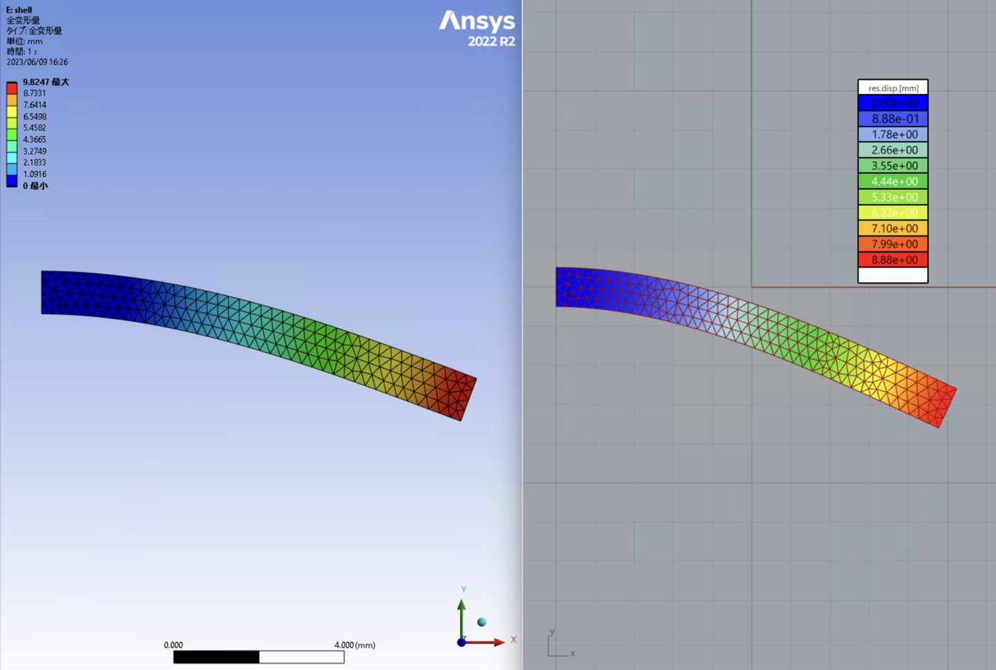
皆さんKaramba3dは好きですか?私はとても好きで愛用しています。
Karamba3dは3D CADのRhinocerosのノードエディタ"Grasshopper"で動く構造解析プラグインです。
このプラグインはRhinocerosのモデリング機能と密接に結びついているため、1つのソフト内で複雑形状をパラメトリックに作成し、それをそのまま構造解析できる点が非常に強い特徴となっている構造解析ソフトです。
公式サイトを見るとサンプルファイルもかなり充実しており、Karamba3dを使った解析のやり方がわからない場合にも参考が多く非常に助かります。
解析ソフトで気になるのは解析の性能です。Karamba3dはAnsysのようなの有名な商用CAEソフトではないため、例えば精度について気になります。
しかしこういった情報はあまり見ないため、本記事では簡単なモデルを対象に確認していきます。
比較対象
Karamba3dのBeam要素とShell要素を、AnsysのShell要素とSolid要素と比較します。
モデル化
ソルバーの違いのみを確認できるよう、極力パラメータは揃えて解析を実施します。
パラメータ
- ヤング率: \(2.0×10^5 \textrm{N/mm}^2\)
- ポアソン比:0.3
- 長さ:10.0mm
- 密度:\(7.85 \textrm{g/cm}^3\)
- メッシュサイズ:0.25mm程度になるようにメッシング、梁要素も0.25mm程度に分割
- 断面:1mm × 1mm の矩形
- 梁ならば矩形断面、シェルならば1mmの板厚を与えています。
メッシュは以下のものを使用しています。Ansysは四角形要素も使うことができますが、Karamba3dは三角形要素しか扱えないため、条件を揃えるために三角形要素のみで比較しています。

比較パターン
以下の8パターンで解析を実施し、結果を比較します。
- Karamba3d
- Beam要素(KrBe)
- Shell要素 面内曲げ (KrSh-in)
- Shell要素 面外曲げ (KrSh-out)
- Ansys
- Shell要素 面内曲げ 1次要素(AnSh1-in)
- Shell要素 面内曲げ 2次要素(AnSh2-in)
- Shell要素 面外曲げ 1次要素(AnSh1-out)
- Shell要素 面外曲げ 2次要素(AnSh2-out)
- Solid要素 6面体2次要素(AnSol)
片持ち梁の先端荷重
では実際に解析を行っていきます。
境界条件
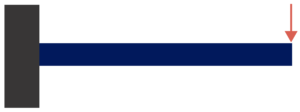
以下のように基端を固定、先端に荷重をかける片持ち梁の問題を解きます。
解析時間の計測
Karamba3dは解析速度が高速ということが知られていますので、その点も比較できるように、解析時間についても確認します。
解析時間は以下の値を使用しています。
- Ansysの解析時間:Elapsed time spent computing solution の値
- Karamba3dの解析時間:解析実施のコンポーネントの処理にかかった時間
- 線形解析であれば Analyze(Karamba3D)
線形静解析
予想値は以下の式で求めています。
荷重の値\(P\)は500Nとしています。
\(\delta = \frac{PL^3}{3EI}, \quad
\sigma = \frac{M}{Z}\)
解析結果
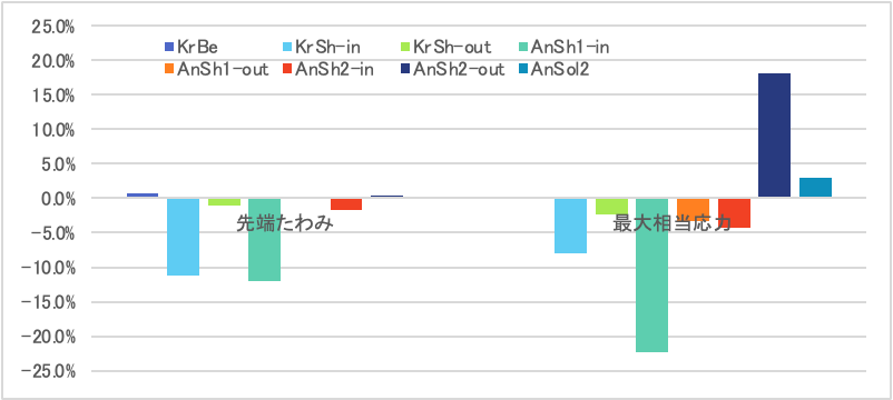
解析結果は以下になりました。
| 微小変形 | KrBe | KrSh-in | KrSh-out | AnSh1-in | AnSh1-out | AnSh2-in | AnSh2-out | AnSol | 予測値 |
|---|---|---|---|---|---|---|---|---|---|
| 先端たわみ [mm] | 10.1 | 8.9 | 9.9 | 8.8 | 10.0 | 9.8 | 10.0 | 10.0 | 10 |
| 予測値との差 | 0.8% | -11.2% | -1.1% | -12.0% | 0.1% | -1.8% | 0.3% | 0.3% | - |
| 最大相当応力 [MPa] | 30000 | 27608 | 29276 | 23302 | 29026 | 28732 | 35425 | 30914 | 30000 |
| 予測値との差 | 0.0% | -8.0% | -2.4% | -22.3% | -3.2% | -4.2% | 18.1% | 3.0% | - |
| 計算時間 [s] | 0.004 | 0.013 | 0.014 | 0.1 | 0.1 | 0.1 | 0.1 | 0.5 | - |
| 計算時間比 | -99.2% | -97.4% | -97.2% | -80.0% | -80.0% | -80.0% | -80.0% | - | - |
Karamba3dのShell要素は1次要素に分類されるもので、結果を見るとAnsysの1次要素と同程度の精度を持っていましたが、2次要素程の精度はない事がわかりました。
計算時間についてはAnsys側の表示が1/10秒までのため、細かな比較はできていませんが、Karamba3dのほうが高速に結果が得られています。
なお表中の数字は読みやすいように丸めていますが、比率の計算は実際の解析から得られた桁数を使っています。
大変形解析
次に大変形解析です。Karamba3dではAnalyze Nonlinear WIPを使用しています。
荷重などの境界条件は同様としています。
使うソルバーを大変形ソルバーにしたのみが差になります
解析結果
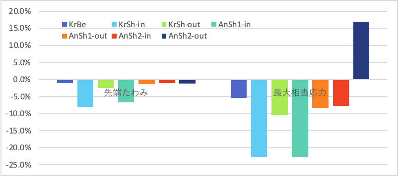
大変形については予測値を求めていないため、表中の比率はAnsysのソリッド要素の結果との差を示しています。
| 大変形 | KrBe | KrSh-in | KrSh-out | AnSh1-in | AnSh1-out | AnSh2-in | AnSh2-out | AnSol |
|---|---|---|---|---|---|---|---|---|
| 先端たわみ [mm] | 6.60 | 6.13 | 6.50 | 6.23 | 6.58 | 6.60 | 6.59 | 6.67 |
| 予測値との差 | -1.1% | -8.0% | -2.5% | -6.6% | -1.4% | -1.0% | -1.2% | - |
| 最大相当応力 [MPa] | 22300 | 18200 | 21100 | 18235 | 21607 | 21747 | 27546 | 23564 |
| 予測値との差 | -5.4% | -22.8% | -10.5% | -22.6% | -8.3% | -7.7% | 16.9% | - |
| 計算時間 [s] | 0.15 | 0.41 | 0.52 | 0.9 | 1.2 | 1.2 | 1.5 | 24.5 |
| 計算時間比 | -99.4% | -98.3% | -97.9% | -96.3% | -95.1% | -95.1% | -93.9% | - |
ねじり荷重
片持ち梁の曲げについて確認したので、次に梁の先端へねじりモーメントを与えたときの結果について確認していきます。
境界条件
以下のように梁の先端をねじる荷重を設定します。

Karamba3dは節点へのモーメント荷重はありますが、先端の複数の節点に対して剛体接続やMPC設定し、中心の節点にモーメントを与える機能はありません。
そのためKaramba3dのシェル要素でねじり荷重をかける際は、先端が一様にねじれるように先端に剛な梁要素を設けてその中心にモーメントをかけています。
AnsysのモデルについてはMPCを設定して、断面の中心に対してモーメントをかけています。
荷重の値は20Nmmとしています。
解析結果
結果は以下のようになります。微小変形で解析を行っています。
ここから、Karamba3dのシェル要素はねじりが硬いことがわかります。
解析時間については、線形解析なので先端荷重時と大きく変わらないことが想定されるため省略しました。
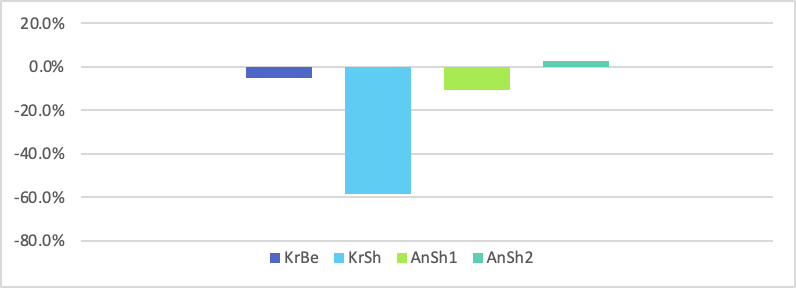
| ねじり | KrBe | KrSh | AnSh1 | AnSh2 | AnSol |
|---|---|---|---|---|---|
| 先端ねじり角 [deg] | 1.01 | 0.44 | 0.94 | 1.09 | 1.06 |
| ソリッドとの差 | -5.1% | -58.3% | -10.8% | 2.6% | - |
固有値解析
Karamba3dは固有値解析も行うことができます。
これまでの静解析でわかった剛性のモデル化に加え、質量も含めたモデル化について確認するため、固有値解析も実施しました。
予測値の計算
各予測値は以下の式で求めています。添字が\(b\)のものが曲げに関する固有振動数、\(t\)のものがねじりに関する固有振動数になります。
なお、ねじり定数\(J\)は対象が矩形断面であることから下式の近似値を使っています。
\(n_{b1} = \frac{1.875^2}{2\pi L^2}\sqrt{\frac{gEI}{\rho A}}, \\
n_{b2} = \frac{4.694^2}{2\pi L^2}\sqrt{\frac{gEI}{\rho A}}, \\
n_{b3} = \frac{7.855^2}{2\pi L^2}\sqrt{\frac{gEI}{\rho A}}, \\
n_{t1} = \frac{\pi}{2L}\sqrt{\frac{gGJ}{\rho I_p}}, J = \frac{0.422}{3}a^4\)
境界条件について
境界条件は、これまで行ってきた解析と同様に基端を固定としています。
解析時間について
固有値の解析時間は10個のモードを抽出するまでの時間としました。
解析結果
結果は以下のようになります。
結果は面内の曲げ、面外の曲げ、それぞれの1次と2次モードとねじりの1次モードの合計5つの固有値について比較しました。
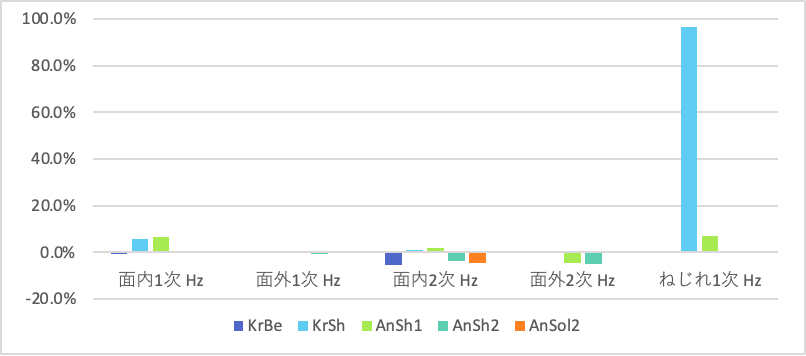
上のグラフではねじり以外の結果が分かりづらいため、拡大したものが以下です。
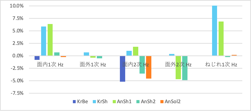
| 固有値 | KrBe | KrSh | AnSh1 | AnSh2 | AnSol | 予測値 |
|---|---|---|---|---|---|---|
| 面内1次 [Hz] | 8089 | 8633 | 8673.8 | 8210 | 8132 | 8153 |
| 予測値との差 | -0.8% | 5.9% | 6.4% | 0.7% | -0.3% | - |
| 面外1次 [Hz] | - | 8208 | 8123.5 | 8113 | - | - |
| 予測値との差 | - | 0.7% | -0.4% | -0.5% | - | - |
| 面内2次 [Hz] | 48441 | 51603 | 52038 | 49277 | 48770 | 51097 |
| 予測値との差 | -5.2% | 1.0% | 1.8% | -3.6% | -4.6% | - |
| 面外2次 [Hz] | - | 51305 | 48710 | 48609 | - | - |
| 予測値との差 | - | 0.4% | -4.7% | -4.9% | - | - |
| ねじり1次 [Hz] | 71917 | 141487 | 76824 | 71712 | 72020 | 71896 |
| 予測値との差 | 0.0% | 96.8% | 6.9% | -0.3% | 0.2% | - |
| 計算時間 [s] | 0.012 | 0.036 | 0.3 | 0.3 | 0.6 | - |
| 計算時間比 | -98.0% | -94.0% | -50.0% | -50.0% | - | - |
固有値解析結果からもわかりますが、曲げについてはAnsysの1次要素程度の精度であることに対して、ねじり荷重時の解析と同様にKaramba3dのシェル要素はねじりが硬いことがわかります。
まとめ
より正確に調べるためにはメッシュの分割数を変化させたり、解析速度の測定は1度ではなく複数回行った値を確認するなどの必要があリますが、概ねの傾向は本記事でわかります。
Karamba3dの梁要素については高い精度、シェル要素については必ずしも予測値に近い値でないこと、解析速度については非常に高速であることがわかったと思います。
そもそもGrasshopperで構造解析を実施する場合の多くは、初期検討でのパラメータースタディなどの多くの解析モデルを高速に回したいという状況なのではないでしょうか。
そのような状況を考えれば、初期検討において十分な精度で非常に高速という特徴はGrasshopperでの構造解析用途の需要にとても合致しています。
結果が予測値とピッタリ合わないからだめではなく、弊社ではこういった知見を元に、各設計内容やフェーズごとに求められるレベルに合わせた適切なソフトを選択することで、より良い設計を目指しています。
補足
Karamba3dのShell要素について興味がある方は、Karamba3dの公式サイトに記載のある以下の論文を参照してください。
- Tric: a simple but sophisticated 3-node triangular element based on 6 rigid.body and 12 straining modes for fast computational simulations of arbitrary isotropic and laminated composite shells.
- J.H. Argyris, L. Tenek, and L. Olofsson.
- Comput. Methods Appl. Mech. Engrg., 145:11–85, 1997
- The tric shell element: theoretical and numerical investigation.
- J.H. Argyris, M. Papadrakakis, C. Apostolopoulou, and S. Koutsourelakis.
- Comput. Methods Appl. Mech. Engrg., 182:217–245, 2000
Do you people like Karamba3d? I like it very much and use it a lot.
Karamba3d is a structural analysis plug-in that runs in the Rhinoceros node editor "Grasshopper".
The plug-in is closely tied to the modeling functionality of Rhinoceros, so it can parametrically create complex geometries and perform structural analysis directly within the software, which is a very strong feature of this structural analysis software.
The official website has a fairly extensive collection of example files, which can be very helpful as a reference if you want to perform an analysis using Karamba3d but don't know how to do it.
One of the main concerns with analysis software is the performance of the analysis, and since Karamba3d is not a well-known commercial CAE software like Ansys, for example, we are concerned about the accuracy of the analysis.
However, since this kind of information is not often available, this article will check it for a simple model.
Subject of comparison
Compare Karamba3d's Beam and Shell elements with Ansys' Shell and Solid elements.
Modeling
The analysis is performed with parameters aligned as much as possible so that only solver differences can be identified.
Parameters
- Young's modulus: \(2.0×10^5 \textrm{N/mm}^2\)
- Poisson's ratio: 0.3
- Length: 10.0 mm
- Density: \(7.85 \textrm{g/cm}^3\)
- Mesh size: Meshing to be about 0.25 mm, beam elements also divided about 0.25 mm
- Cross section: 1mm × 1mm rectangle
- A rectangular cross-section is given for beams, and a thickness of 1mm for shells.
The meshes used are as follows: Ansys can also use quad elements, but Karamba3d can only handle triangles, so to keep the conditions consistent, only triangles are used for comparison.
Comparison Patterns
The following 8 patterns are used to perform the analysis and compare the results.
- Karamba3d
- Beam element (KrBe)
- Shell element In-plane bending (KrSh-in)
- Shell element out-of-plane bending (KrSh-out)
- Ansys
- Shell element in-plane bending 1st order element (AnSh1-in)
- Shell element in-plane bending 2nd order element (AnSh2-in)
- Shell element out-of-plane bending 1st order element (AnSh1-out)
- Shell element out-of-plane bending 2nd order element (AnSh2-out)
- Solid element Hexahedron 2nd order element (AnSol)
Cantilevered beam tip load
Now we will actually perform the analysis.
Boundary conditions
We will solve the following problem for a cantilevered beam with a fixed base end and a load applied at the tip.
Measuring analysis time
Since Karamba3d is known for its high analysis speed, we will also check the analysis time so that we can compare that as well.
The following values are used for analysis time.
- Ansys analysis time: "Elapsed time spent computing solution" value
- Karamba3d analysis time: Elapsed time spent processing the components of the analysis
- Analyze(Karamba3D) for linear analysis
Linear static analysis
The predicted value is obtained by the following equation.
The value of the load \(P\) is set to 500N.
\(\delta = \frac{PL^3}{3EI}, \quad
\sigma = \frac{M}{Z}\)
Analysis Results
The results of the analysis are as follows
| KrBe | KrSh-in | KrSh-out | AnSh1-in | AnSh1-out | AnSh2-in | AnSh2-out | AnSol | Predicted | |
|---|---|---|---|---|---|---|---|---|---|
| Tip deformation [mm] | 10.1 | 8.9 | 9.9 | 8.8 | 10.0 | 9.8 | 10.0 | 10.0 | 10 |
| Diff | 0.8% | -11.2% | -1.1% | -12.0% | 0.1% | -1.8% | 0.3% | 0.3% | - |
| Max VonMises [MPa] | 30000 | 27608 | 29276 | 23302 | 29026 | 28732 | 35425 | 30914 | 30000 |
| Diff | 0.0% | -8.0% | -2.4% | -22.3% | -3.2% | -4.2% | 18.1% | 3.0% | - |
| Computing Time [s] | 0.004 | 0.013 | 0.014 | 0.1 | 0.1 | 0.1 | 0.1 | 0.5 | - |
| Diff | -99.2% | -97.4% | -97.2% | -80.0% | -80.0% | -80.0% | -80.0% | - | - |
Karamba3d's Shell element is classified as a 1st order element, and the results show that it has the same level of accuracy as Ansys' 1st order element, but not as accurate as the 2nd order element.
The calculation time is not compared in detail because the Ansys display is limited to 1/10th of a second, but Karamba3d is faster than Ansys.
The numbers in the table are rounded for readability, but the ratios are calculated using the number of digits obtained from the actual analysis.
Large Deformation Analysis
Next, we will perform a large deformation analysis using Analyze Nonlinear WIP in Karamba3d.
The boundary conditions such as load are the same.
The only difference is that the solver used is a large-form solver.
Analysis Results
Since predictions were not calculated for large deformations, the percentages in the table show the difference from the results of Ansys solid elements.
| KrBe | KrSh-in | KrSh-out | AnSh1-in | AnSh1-out | AnSh2-in | AnSh2-out | AnSol | |
|---|---|---|---|---|---|---|---|---|
| Tip deformation [mm] | 6.60 | 6.13 | 6.50 | 6.23 | 6.58 | 6.60 | 6.59 | 6.67 |
| Diff | -1.1% | -8.0% | -2.5% | -6.6% | -1.4% | -1.0% | -1.2% | - |
| Max Von Mises [MPa] | 22300 | 18200 | 21100 | 18235 | 21607 | 21747 | 27546 | 23564 |
| Diff | -5.4% | -22.8% | -10.5% | -22.6% | -8.3% | -7.7% | 16.9% | - |
| Computing time [s] | 0.15 | 0.41 | 0.52 | 0.9 | 1.2 | 1.2 | 1.5 | 24.5 |
| Diff | -99.4% | -98.3% | -97.9% | -96.3% | -95.1% | -95.1% | -93.9% | - |
Torsional Load
Now that we have reviewed the bending of cantilevered beams, we will now review the results when a torsional moment is applied to the end of the beam.
Boundary conditions
Set the torsion load to the tip of the beam as follows.
Karamba3d has moment loading on nodes, but it does not have the ability to set rigid connections or MPC for multiple nodes at the tip and apply moment to the center node.
Therefore, when applying a torsional load to a Karamba3d shell element, a rigid beam element is set at the tip and the moment is applied to the center of the beam element so that the tip twists uniformly.
For the Ansys model, MPC is set up and the moment is applied to the center of the cross section.
The value of the load is set to 20 Nmm.
Analysis Results
The results are as follows.
From this we can see that the Karamba3d shell element is torsionally stiffer.
The analysis time was omitted because it is a linear analysis and is not expected to be significantly different from that for tip loading.
| KrBe | KrSh | AnSh1 | AnSh2 | AnSol | |
|---|---|---|---|---|---|
| Tip torsion angle [deg] | 1.01 | 0.44 | 0.94 | 1.09 | 1.06 |
| Diff | -5.1% | -58.3% | -10.8% | 2.6% | - |
Eigenvalue Analysis
Karamba3d can also perform eigenvalue analysis.
In addition to the modeling of stiffness found in the static analysis so far, eigenvalue analysis was also performed to confirm the modeling of mass as well.
Calculation of predicted values
Each predicted value is calculated by the following equation. The values with subscript \(b\) are the natural frequencies for bending, and those with subscript \(t\) are the natural frequencies for torsion.
The torsion constant \(J\) is an approximation of the following equation, since the object is a rectangular cross section.
\(n_{b1} = \frac{1.875^2}{2\pi L^2}\sqrt{\frac{gEI}{\rho A}}, \\
n_{b2} = \frac{4.694^2}{2\pi L^2}\sqrt{\frac{gEI}{\rho A}}, \\
n_{b3} = \frac{7.855^2}{2\pi L^2}\sqrt{\frac{gEI}{\rho A}}, \\
n_{t1} = \frac{\pi}{2L}\sqrt{\frac{gGJ}{\rho I_p}}, J = \frac{0.422}{3}a^4\)
Boundary conditions
The boundary conditions are fixed at the base end as in the previous analyses.
Analysis time
The analysis time for eigenvalues is the time required to extract 10 modes.
Analysis Results
The results are shown below.
Results were compared for a total of five eigenvalues: in-plane bending, out-of-plane bending, first and second order modes of each, and first order mode of torsion.
Since it is difficult to see results other than torsion in the above graph, an enlarged version is shown below.
| KrBe | KrSh | AnSh1 | AnSh2 | AnSol | Predicted | |
|---|---|---|---|---|---|---|
| In-plan 1st [Hz] | 8089 | 8633 | 8673.8 | 8210 | 8132 | 8153 |
| Diff | -0.8% | 5.9% | 6.4% | 0.7% | -0.3% | - |
| Out-plan 1st [Hz] | - | 8208 | 8123.5 | 8113 | - | - |
| Diff | - | 0.7% | -0.4% | -0.5% | - | - |
| In-plane 2nd [Hz] | 48441 | 51603 | 52038 | 49277 | 48770 | 51097 |
| Diff | -5.2% | 1.0% | 1.8% | -3.6% | -4.6% | - |
| Out-plane 2nd [Hz] | - | 51305 | 48710 | 48609 | - | - |
| Diff | - | 0.4% | -4.7% | -4.9% | - | - |
| Tosion 1st [Hz] | 71917 | 141487 | 76824 | 71712 | 72020 | 71896 |
| Diff | 0.0% | 96.8% | 6.9% | -0.3% | 0.2% | - |
| Computing time [s] | 0.012 | 0.036 | 0.3 | 0.3 | 0.6 | - |
| Diff | -98.0% | -94.0% | -50.0% | -50.0% | - | - |
As can be seen from the eigenvalue analysis results, the Karamba3d shell element is torsionally stiff, as is the analysis under torsional loading, while for bending it is as accurate as an Ansys first-order element.
Conclusion
To get a more accurate result, it is necessary to check the values by changing the number of mesh divisions and measuring the analysis speed not once but multiple times.
We have found that Karamba3d is highly accurate for beam elements, not always close to the predicted values for shell elements, and very fast in terms of analysis speed.
In most cases where structural analysis is performed in Grasshopper, there is a need to run a large number of analysis models at high speed, such as parameter studies in the initial study.
Considering such a situation, the feature of being very fast with sufficient accuracy in the initial study is very much in line with the demand for structural analysis applications in Grasshopper.
We aim for better design not because the results do not exactly match the predicted values, but by using this knowledge to select the appropriate software for the level required for each design content and phase.
Appendix.
If you are interested in the Shell element of Karamba3d, please refer to the following paper, which can be found on the official Karamba3d website
- Tric: a simple but sophisticated 3-node triangular element based on 6 rigid.body and 12 straining modes for fast computational simulations of arbitrary isotropic and laminated composite shells.
- J.H. Argyris, L. Tenek, and L. Olofsson.
- Comput. Methods Appl. Mech. Engrg., 145:11–85, 1997
- The tric shell element: theoretical and numerical investigation.
- J.H. Argyris, M. Papadrakakis, C. Apostolopoulou, and S. Koutsourelakis.
- Comput. Methods Appl. Mech. Engrg., 182:217–245, 2000
