
弊社の廣谷、新谷、古澤と、大阪大学大学院工学研究科の矢地謙太郎准教授による、冷却流路のトポロジー最適化手法に関する共著論文が国際学術誌Structural and Multidisciplinary Optimization(SMO)に採択されました[1]。本記事では論文の内容や思想をなるべくわかりやすく解説したいと思います。
はじめに
トポロジー最適化は人間が思いもよらないような設計の示唆を与えてくれるものであり、より良い製品を設計する上で有効な手法です[2]。
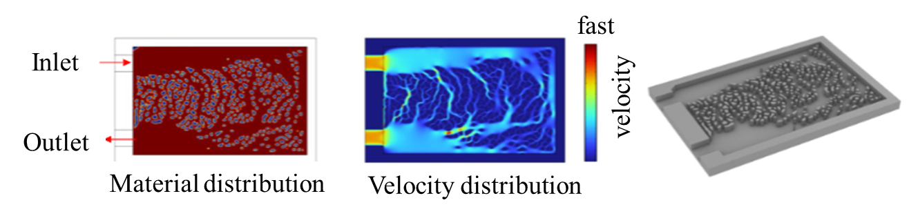
トポロジー最適化手法の中でも、密度法に基づくトポロジー最適化は一般的に広く用いられており、構造分野のみならず熱流体分野をはじめとして多分野に適用されています[3]。
冷却流路への密度法に基づくトポロジー最適化適用例
しかし、最適化結果が複雑形状になることがしばしばあり、物理的解釈や製造への落とし込み、製造品質の管理に課題が残ります。
密度法に基づくトポロジー最適化においてもフィルタを用いて部材寸法を間接的に制御することは可能ですが、複雑な設計制約を最適化結果に厳密に反映させるのは困難です。
既存の製造技術を前提とした実用的な設計解を得るためには、最適化結果を設計者が読み取り、最適性を損なわないように細心の注意を払いつつ製造可能な形状へと調整する後処理が必要です。
また、最適化結果をCADモデルに変換する際にもグレースケールを含む密度画像から明瞭なCADモデルへ変換するための後処理が不可欠です。
本研究では、寸法等の幾何学的な設計制約を柔軟に組み込めるほか、得られた形状の物理的な意味を解釈しやすく、最適化後の形状調整にも繋げやすい冷却流路のトポロジー最適化手法を提案しました。
Moving Morphable Components(MMC)
トポロジー最適化手法の一つにMoving Morphable Components(MMC)があります[4]。

Moving Morphable Components(MMC)の概念図
Moving Morphable Components(MMC)は、解析に用いる有限要素とは別に、あらかじめ最適幾何形状の部材となり得る要素を「構成要素」として設計領域に配置しておき、構成要素の移動、回転、拡大、縮小、重ね合わせで幾何形状を表現する手法です。
MMCの定式化の概説や構造ベンチマーク問題に適用した結果については過去の記事をご覧ください。
トポロジー最適化手法の概要と比較 | Nature Architects inc.
MMCでは、構成要素の寸法・位置・角度といった形状情報を設計変数として直接的に制御できるため、
- 「この部材の厚みは特定の範囲に制限する」
- 「この構成要素は指定した領域内でのみ移動可能にする」
- 「この隣接する構成要素間はC¹連続性を保つ[5]」
などといったような幾何学的な制約を最適化へ厳密に組み込むことが可能です。
さらに、設計変数が形状パラメタそのものであるため、最適化結果をシームレスにCADシステムへ移行できるという実務上の利点も備えています。
提案する冷却流路最適化フレームワークの概要
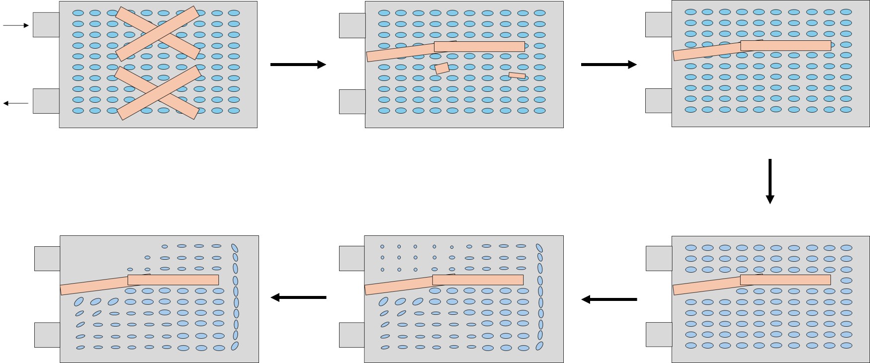
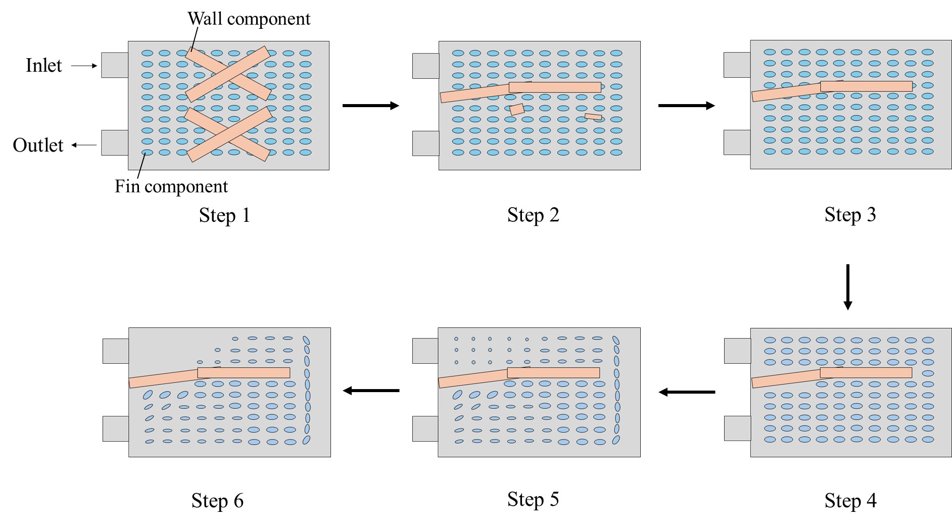
本研究では、大域的流路を形成する「壁」と局所的な熱伝達を促進する「フィン」という異なる物理的な役割を割り当てられた構成要素を定義し、役割ごとに最適化段階を分けることで、両者の競合を抑えながら設計できる二段階最適化手法を提案しました。手法の概念図は下図の通りです。
提案する二段階最適化手法の概念図
-
Step 1:設計領域内に、壁構成要素とフィン構成要素を配置する
Step 2:壁構成要素のみを設計変数として、大域的な流路ネットワークを最適化する
Step 3:最適化後の壁構成要素のうち、寸法が所定のしきい値を下回る大域的な流路の形成に寄与しないものを削除する
Step 4:残された壁構成要素に対して、所定のしきい値距離よりも近くに位置するフィン構成要素を削除し、第2段階の最適化に用いるフィン候補のみを残す
Step 5:残されたフィン構成要素のみを設計変数として、流路内の局所的な熱伝達特性を最適化する
Step 6:最後に、寸法が所定のしきい値を下回るフィン構成要素を削除し、得られた構造を最終設計として採用する
具体的な最適化プロセスは上記のStep 1~Step 6です。
物理的な役割に応じて最適化段階を分けつつ、最適化段階の合間に、意図にそぐわない構成要素を枝刈りすることにより、設計意図に沿った製造のしやすい結果を得ることが可能となります。
熱流体解析モデル
本研究では、冷却流体と流路壁を含む上部熱流体層と、発熱体からの熱を受ける下部基板層からなる二層熱流体モデルを用いています[6]。
本来は三次元的な流れと熱伝達を、厚さ方向の速度・温度分布を仮定して二次元問題に縮約することで、トポロジー最適化に必要な多数回の解析を効率的に行います。
上部熱流体層では、非圧縮性流体の流れを仮定し、連続の式を解きます。
ここで、\(\mathbf{u}\)は面内方向の流速です。
運動量保存則には、固体領域内の流れを抑制するBrinkman抵抗を加えた次式を用います。
右辺最後の \(-\alpha(\gamma)\mathbf{u}\)がBrinkman抵抗です。
流体領域では抵抗を小さく、固体領域では抵抗を大きくすることで、流路と壁を同じ方程式の中で表現します。
上部熱流体層の温度\(T_t\)については、流れによる熱輸送、面内方向の熱伝導、下部基板層との熱交換を考慮します。
第1項は流体による熱の移流、第2項は熱伝導、第3項は上部熱流体層と下部基板層の間の熱移動を表します。
下部基板層では流れを考慮せず、基板内の熱伝導を次式で計算します。
ここで、\(T_b\)は基板層の代表温度、\(q_0^{\prime\prime}\) は発熱体から与えられる熱流束です。
発熱体から基板へ入力された熱は、基板内を伝導した後、上部の流体または流路壁へ移動します。
MMC構成要素の数学的表現と物性値への反映
MMCでは、壁やフィンを形状明示的な構成要素として表現し、その位置・寸法・角度を設計変数とします。一方、熱流体解析では、固定された有限要素メッシュ上の各位置が流体であるか固体であるかを、材料分布 \(\gamma\) によって表す必要があります。
そこで本研究では、次の流れでMMC構成要素の形状を熱流体解析の物性値へ反映します。
ここで、\(\alpha(\gamma)\)は流体抵抗、\(k_t(\gamma)\) は上部熱流体層の実効熱伝導率、\(h(\gamma)\) は上下層間の熱伝達係数です。
壁構成要素のTDF
設計領域内の任意の点を \((X,Y)\)、壁構成要素の中心座標を \((X_0,Y_0)\) とします。まず、壁構成要素の向きに合わせた局所座標を次のように定義します。
ここで、\(s_w\) は壁の長手方向、\(n_w\) は長手方向に直交する方向の局所座標であり、\(\theta\) は壁構成要素の回転角です。
壁構成要素の形状は、6次の超楕円型TDFによって表されます。
ここで、\(L\)は長手方向の寸法、\(t\)は幅方向の寸法です。
指数を6とすることで、通常の楕円よりも矩形に近い、棒状の壁形状を滑らかな関数として表現しています。
フィン構成要素のTDF
フィン構成要素についても同様に、その中心座標を \((X_f,Y_f)\)として局所座標を定義します。
ここで、\(\psi\)はフィンの回転角です。
楕円形のフィン構成要素は、次のTDFで表されます。
\(a\)は楕円の長半径、\(k\)は短半径と長半径の比であり、短半径 \(b\)は次式となります。
したがって、\(k=1\)の場合は円形となり、\(k\)を小さくすると細長い楕円形になります。
なお、ここでの \(k\)はフィン形状の軸比であり、後述する熱伝導率 \(k_f\)、\(k_s\)とは異なります。
壁とフィンのいずれについても、TDFは次の符号を取ります。
TDFから材料分布への変換
TDFはそのままでは 0 から 1の材料分布として使用できないため、双曲線正接関数を用いて、各TDFをおおむね0から1の範囲に投影します。
壁構成要素の投影TDFは、
フィン構成要素の投影TDFは、
で表されます。
\(\beta\)は、構成要素の境界における流体と固体の切り替わりの鋭さを調整するパラメータです。この定義では、構成要素の内部で投影TDFが0に近づき、構成要素の外部で1に近づきます。
壁とフィンの生のTDFを直接掛け合わせるのではなく、これらを0から1に投影した関数の積から材料分布 \(\gamma\)を求めます。
壁とフィンを統合した材料分布
壁構成要素の集合を \(C_w\)、フィン構成要素の集合を \(C_f\)とすると、設計領域全体の材料分布は次式で表されます。
ここで、\(\mathbf{d}_{w,m}\) と \(\mathbf{d}_{f,n}\) は、それぞれ壁構成要素とフィン構成要素の設計変数です。
本研究における材料分布の定義は、
です。
投影TDFの積を取っているため、ある点が壁またはフィンのいずれか一つの内部に存在すれば、その位置の\(\gamma\)は0に近づき、固体として扱われます。
一方、すべての構成要素の外部にある点では、それぞれの投影TDFが1に近くなるため、\(\gamma\)も1に近づき、流体として扱われます。
したがって、この積は複数の壁・フィン構成要素の固体領域の和集合を表しています。壁とフィンが重なった場合も、その領域は固体となります。
二段階最適化では更新する設計変数のみが切り替わり、第1段階と第2段階のいずれでも、この材料分布の表現自体は共通です。
材料分布から流体抵抗への変換
材料分布 \(\gamma\)は、まずBrinkman抵抗係数 \(\alpha(\gamma)\)に反映されます。流体と固体の間の抵抗値は、RAMP関数を用いて次式で補間されます。
ここで、\(\alpha_f\)は流体領域の抵抗、\(\alpha_s\)は固体領域の抵抗、\(q_f\)は補間関数の非線形性を調整するパラメータです。
両端の値は次のようになります。
流体側と固体側の抵抗値は、それぞれ次式で定義されます。
ここで、\(\mu\)は流体の粘性係数、\(H_t\)は上部熱流体層の半厚さです。
固体領域では流体領域よりも非常に大きな抵抗を与えることで、運動量保存則に含まれるBrinkman抵抗項
によって、壁やフィン内部の流速をほぼゼロにします。一方、\(\gamma\simeq1\)の流路領域では抵抗が小さくなり、流体が流れることができます。
材料分布から熱伝導率への変換
材料分布 \(\gamma\)は、上部熱流体層の実効熱伝導率 \(k_t(\gamma)\)にも反映されます。
ここで、\(k_f\)は流体の熱伝導率、\(k_s\)は固体の熱伝導率、\(q_k\)は補間関数の非線形性を調整するパラメータです。
したがって、流路部分では流体の熱伝導率が使用され、壁やフィンの内部では固体の熱伝導率が使用されます。
最適化途中に現れる中間的な \(\gamma\) に対しては、流体と固体の間の実効的な熱伝導率が与えられます。
材料分布から層間熱伝達係数への変換
上部熱流体層と下部基板層の間の熱伝達係数 \(h(\gamma)\)も、実効熱伝導率 \(k_t(\gamma)\)を介して材料分布に依存します。
上部熱流体層側の熱伝達係数は、
下部基板層側の熱伝達係数は、
で表されます。ここで、\(k_b\)は基板の熱伝導率、\(H_b\)は下部基板層の半厚さです。
上下層を合わせた熱伝達係数は、両層の熱抵抗を直列に接続した形で、
と計算されます。
このため、MMC構成要素の形状が変わって \(\gamma\)が変化すると、流体抵抗だけでなく、上部層の熱伝導率と基板から上部層への熱移動量も変化します。
以上より、MMC構成要素の形状変更は、次の経路で熱流体解析に反映されます。
すなわち、最適化によって壁やフィンの位置・寸法・角度が更新されると、その形状が材料分布 \(\gamma\)に変換され、有限要素ごとの流体抵抗および熱物性が更新されます。
これにより、最適化中に解析メッシュを作り直すことなく、構成要素の形状変化を流れ場と温度場へ反映できます。
最適化問題
最適化対象となる液冷冷却プレート
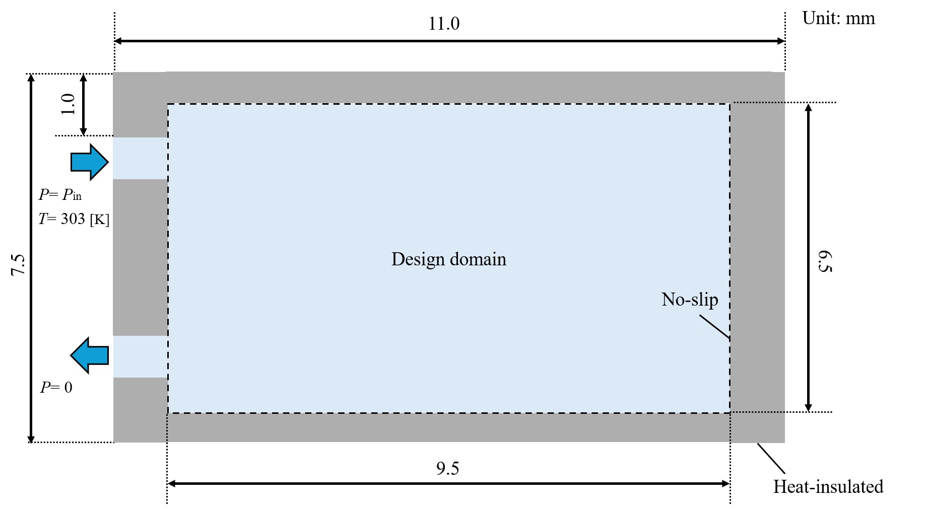
最適化対象は上図に示すような液冷の冷却プレートです。
左上に流入口、左下に流出口があり、流入出口を圧力境界とすることで流体を駆動しています。
流体領域の物性値は水、固体領域の物性値はシリコンを用います。
設計領域全体に一定の熱流速を与えることで、発熱物体を模擬しています。
目的関数は、上式に示すような固体領域温度の\(p\)ノルム平均で、\(p=10\)と設定したため最大温度最小化相当の目的関数となっています。
最適化結果
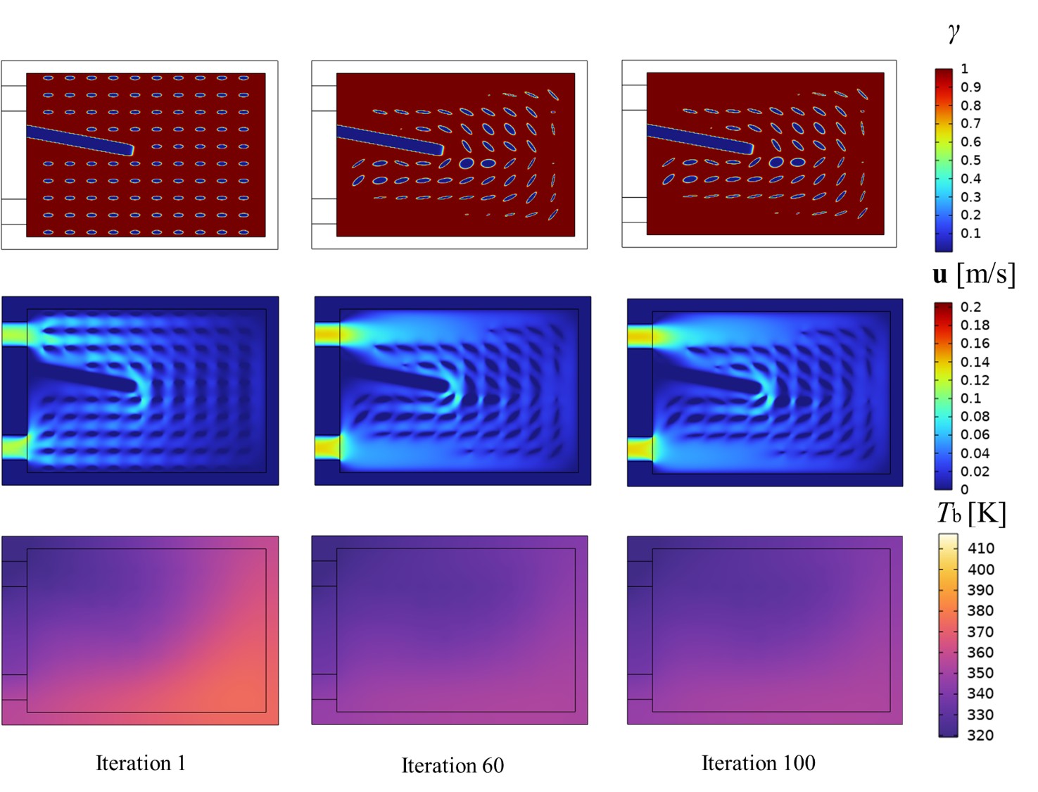
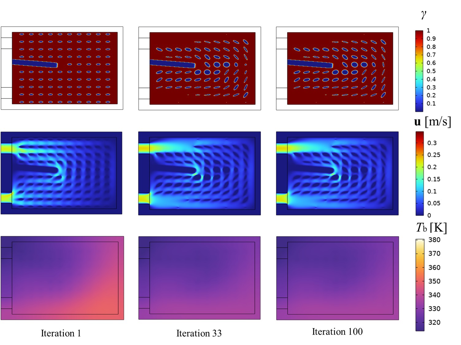
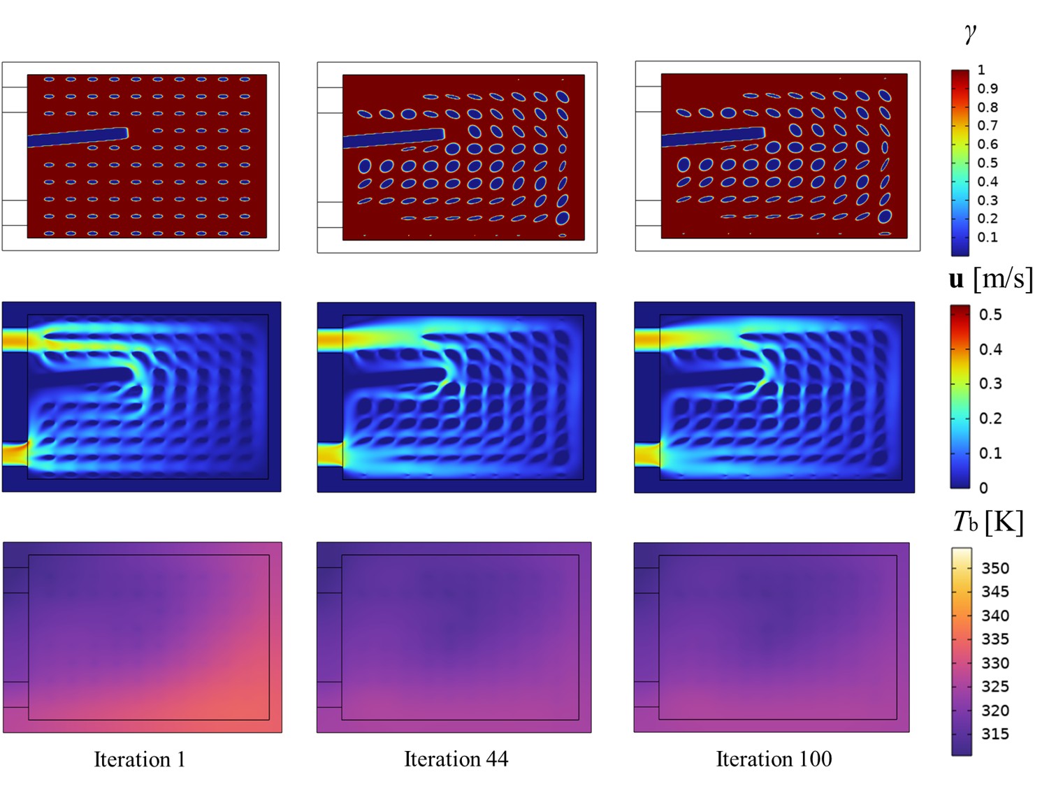
各流入圧力における壁・フィンの最適化結果
本研究では、流入圧力を\(P_{in}= 50、100、200 Pa\) とした3条件について、壁構成要素とフィン構成要素を最適化しました。
壁構成要素の最適化
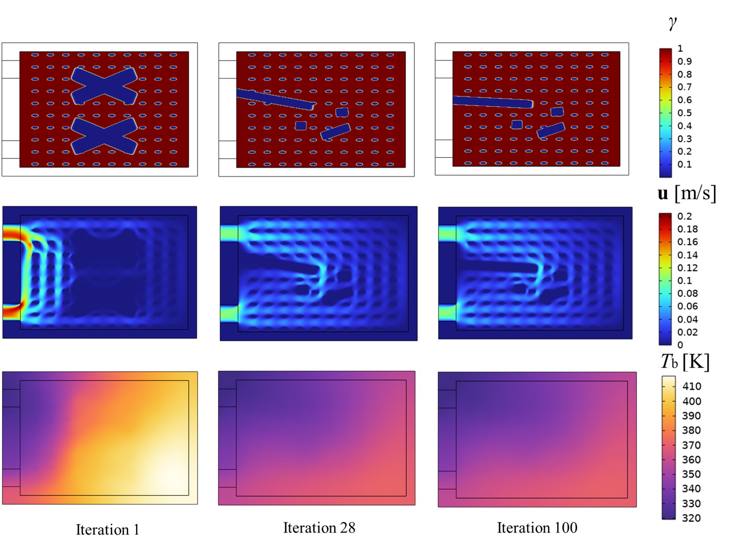
壁構成要素の最適化結果:流入圧力 50 Pa
(a) \(P_{in}=50 Pa\)の結果
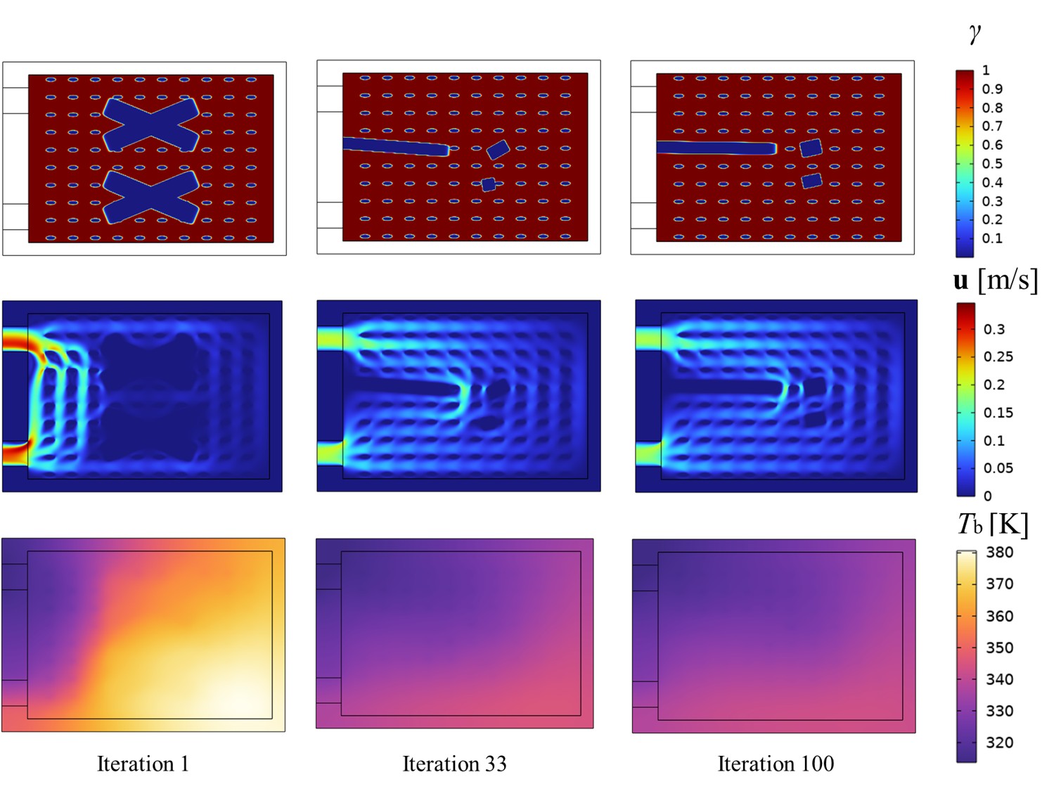
壁構成要素の最適化結果:流入圧力 100 Pa
(b) \(P_{in}=100 Pa\)の結果
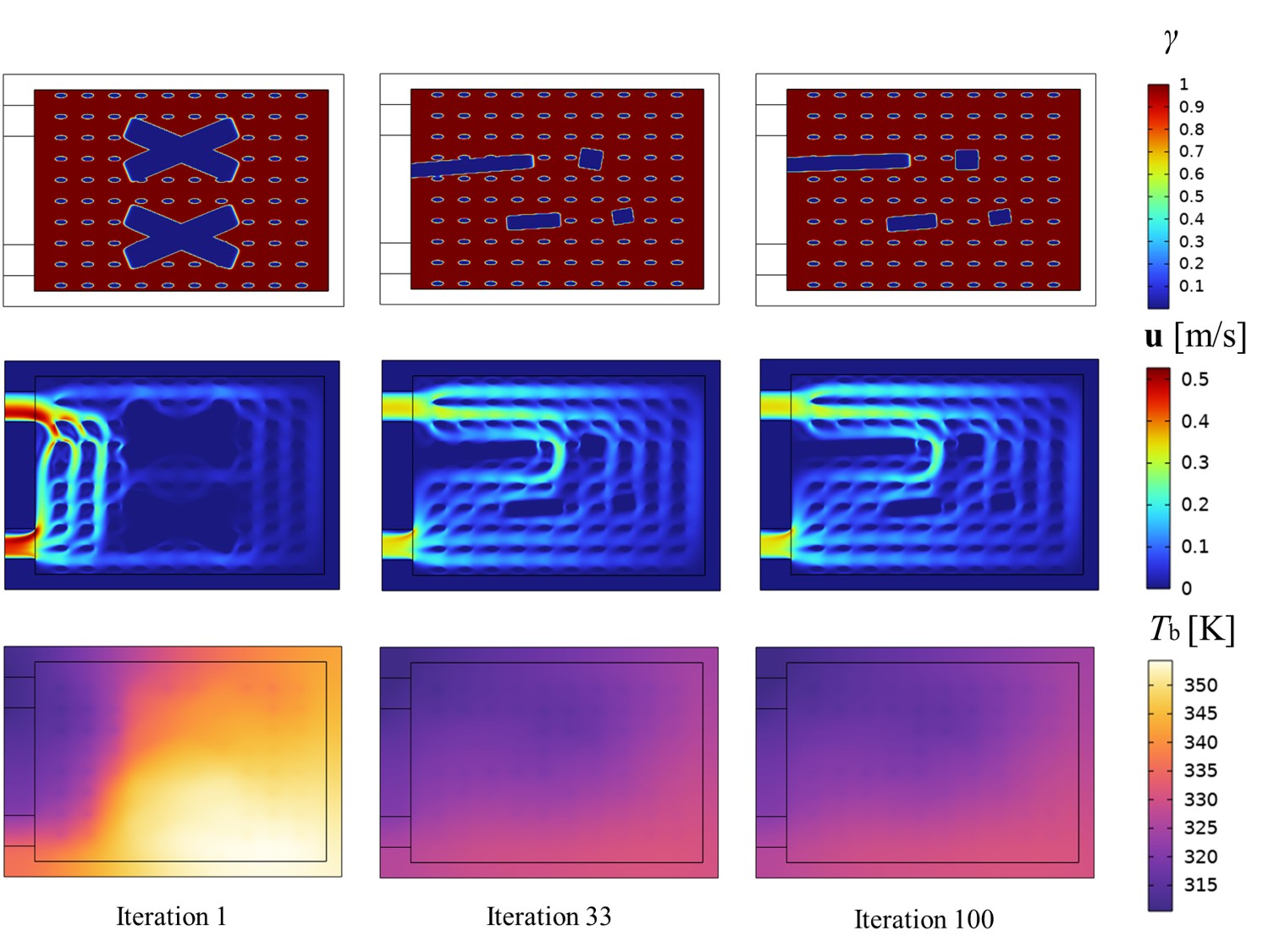
壁構成要素の最適化結果:流入圧力 200 Pa
(c) \(P_{in}=200 Pa\)の結果
上図では、各流入圧力における壁構成要素の最適化過程を示しています。各条件の上段は材料分布、中段は流速分布、下段は基板の温度分布です。
初期形状では、入口から近接する出口へ冷却流体が直接流れやすく、設計領域の右側に十分な流れが届いていません。
最適化が進むと、すべての流入圧力において、この短絡的な流れを遮るように壁構成要素が移動・変形し、冷却流体を設計領域の右側まで迂回させる大域的な流路が形成されました。
その結果、冷却流体がより広い範囲を通過し、基板全体の温度が低下しています。
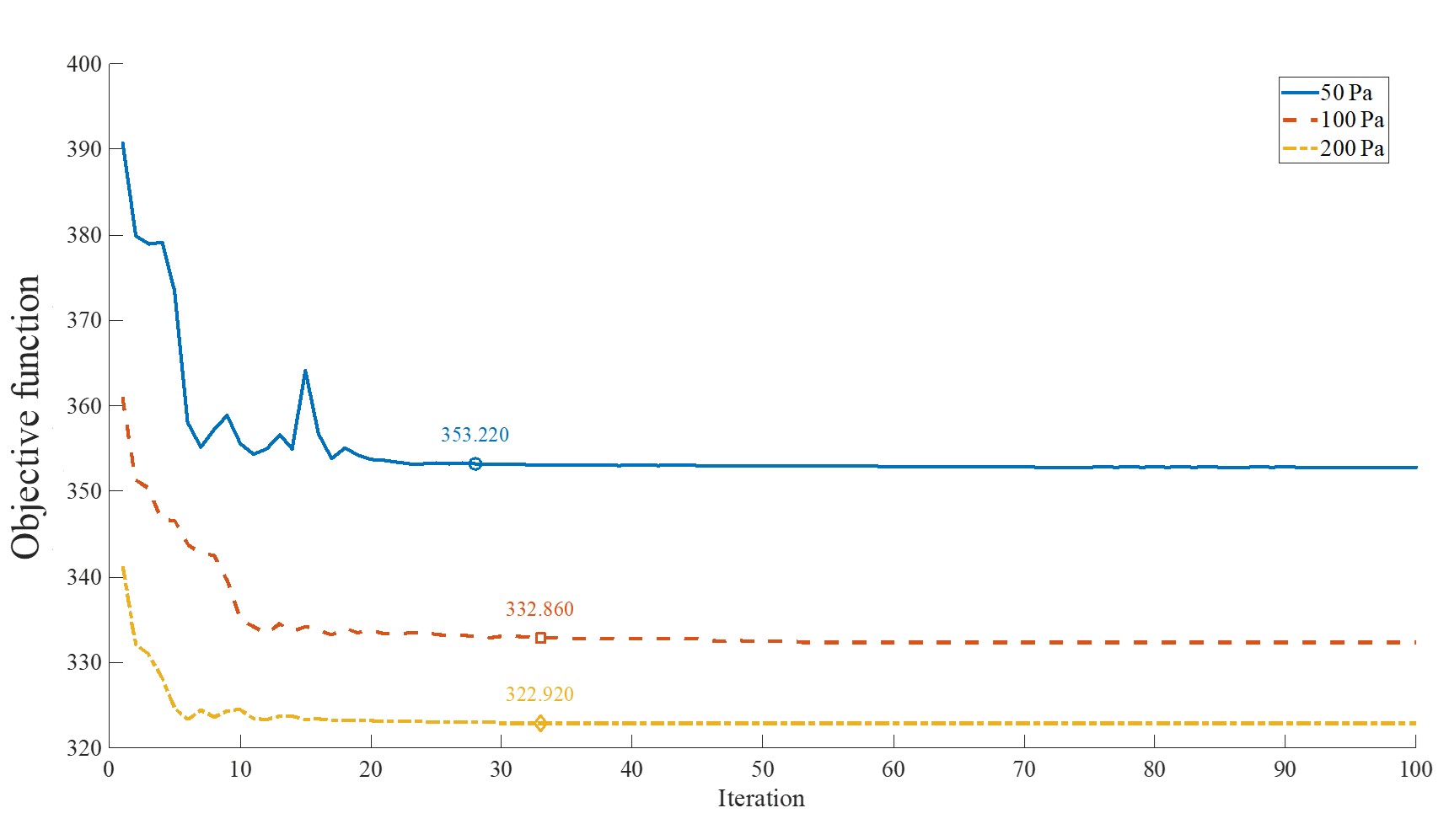
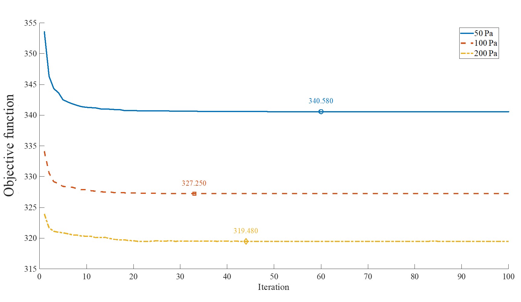
壁構成要素最適化における目的関数履歴
上図の目的関数履歴を見ると、いずれの流入圧力でも最適化初期に目的関数が大きく低下し、その後はほぼ一定値に収束しています。
流入圧力が高いほど流速が大きくなり、対流による熱輸送が強くなるため、最終的な目的関数も小さくなりました。
フィン構成要素の最適化
壁構成要素の最適化後、大域的な流路の形成に寄与しない小さな壁構成要素を除去し、残された流路形状を固定した状態でフィン構成要素を最適化しました。
フィン構成要素の最適化結果:流入圧力 50 Pa
(a) \(P_{in}=50 Pa\)の結果
フィン構成要素の最適化結果:流入圧力 100 Pa
(b) \(P_{in}=100 Pa\)の結果
フィン構成要素の最適化結果:流入圧力 200 Pa
(c) \(P_{in}=200 Pa\)の結果
上図では、フィンの大きさや向きが局所的な流れに応じて変化し、高温領域へ冷却流体を導く形状が形成されています。
すべての流入圧力において、フィンの最適化によって流れが局所的に調整され、壁のみを最適化した場合から冷却性能がさらに向上しました。
一方、最適化後に残るフィンの数や分布は流入圧力によって異なります。
流入圧力が高い場合は、フィンによって生じる流れの曲がりや再循環が流体の混合を促し、温度境界層を薄くすることで熱伝達を高められるため、比較的多くのフィンが残ります。
これに対して流入圧力が低い場合は、対流による熱輸送が弱く、フィンによる流動抵抗の増加が相対的に大きくなるため、フィンはより疎に配置されます。
フィン構成要素最適化における目的関数履歴
上図の通り目的関数も低減できていることがわかります。
密度法に基づくトポロジー最適化との比較
提案手法の性能を評価するため、流入圧力 \(P_{in}=200 Pa\)の条件について、一般的な密度法に基づくトポロジー最適化との比較を行いました。
比較では、熱流体モデル、境界条件、有限要素メッシュ、物性値の補間方法、および初期材料分布を両手法で共通としています。
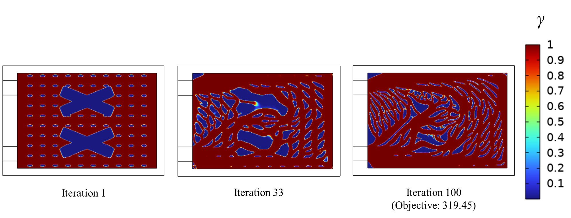
密度法に基づくトポロジー最適化の結果
提案手法が壁とフィンの位置・寸法・向きを設計変数とするのに対し、密度法では有限要素ごとに配置された密度変数を直接更新します。
そのため、密度法は局所的な形状自由度が非常に高く、上図では、多数の細長い形状や複雑な局所構造を含む材料分布が生成されています。
なお、結果に残っている棒状および楕円状の特徴の一部は、両手法で共通化した初期材料分布に由来するものであり、密度法に壁やフィンの幾何学的制約が課されているわけではありません。
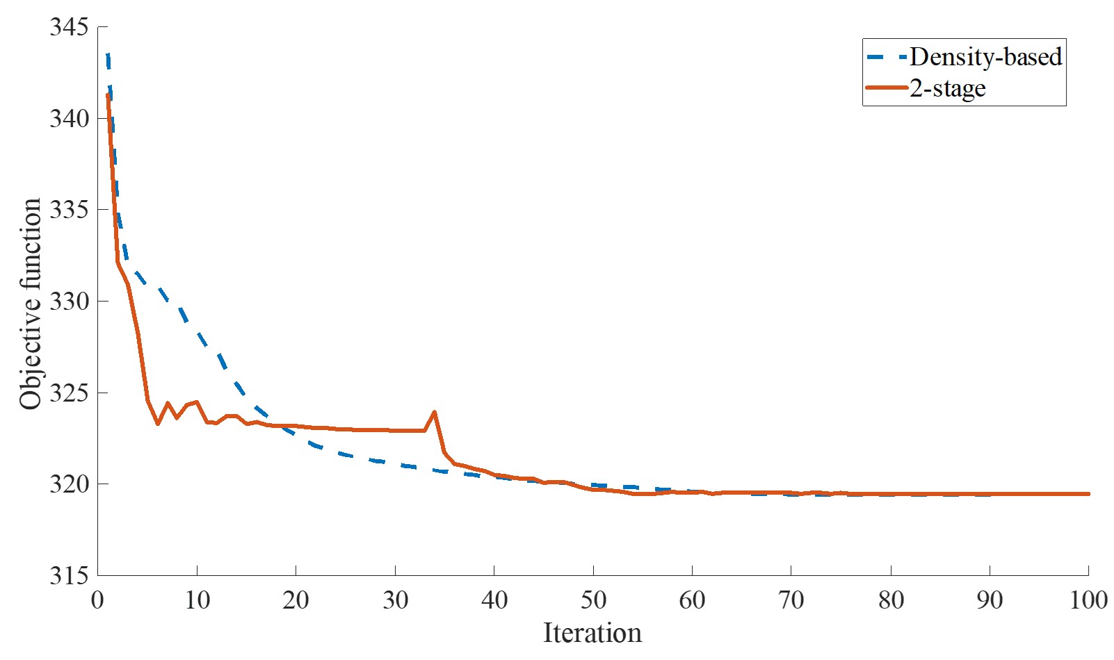
提案手法と密度法における目的関数履歴の比較
上の目的関数履歴を見ると、提案手法では、最初の壁最適化によって目的関数が急速に低下し、最適化段階の切り替え時に一時的な変動を示した後、フィン最適化によってさらに低下しています。
一方、密度法では、すべての密度変数を連続して更新するため、目的関数が比較的滑らかに低下しています。
最終的には、提案手法が約319.48、密度法が約319.40となり、両者はほぼ同等の冷却性能に到達しました。
設計変数の数は、提案手法の299個に対して密度法に基づく最適化では84,480個であり、提案手法は約 1/283 の設計変数で最適化を行っています。
形状表現を壁とフィンに限定して局所的な自由度を大幅に削減しているにもかかわらず、密度法に基づく最適化とほぼ同等の目的関数を達成したことから、設計者が意図した構成要素による形状表現の有効性が確認できます。
この比較の重要な点は、提案手法が密度法より一般的に高い性能を示したということではありません。
密度法基づく最適化に比べて制限された設計空間を用いながら、同程度の冷却性能を維持しつつ、より単純で解釈しやすく、寸法調整などを行いやすい形状を得られたことに意義があります。
壁とフィンの同時最適化との比較
提案する二段階最適化の有効性を確認するため、流入圧力 \(P_{in}=200 Pa\) の条件において、壁構成要素とフィン構成要素を同時に更新する最適化との比較を行いました。
初期形状、目的関数、支配方程式、境界条件、物性値の補間方法、および有限要素メッシュは、二段階最適化と同一です。
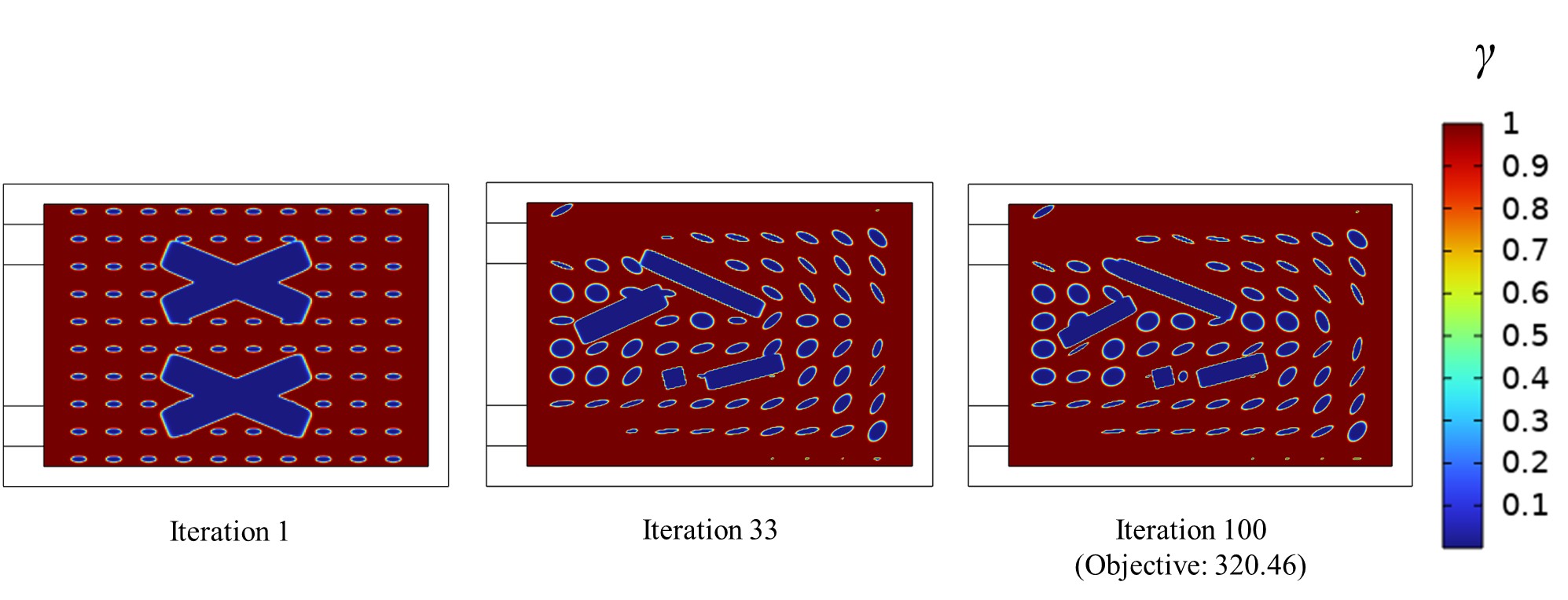
二段階最適化と壁・フィン同時最適化の結果比較
上図に示す同時最適化では、壁とフィンのすべての設計変数を同時に更新します。
その結果、本来は大域的な流路を形成するために導入した壁構成要素の一部が局所的な熱伝達促進に利用され、反対に、フィン構成要素の一部が大域的な流路形成に関与しています。
このように、壁とフィンの機能が互いに混在し、各構成要素が最終形状の中でどのような物理的役割を担っているのかが不明確になりました。
これに対して二段階最適化では、最初に壁構成要素だけで大域的な流路の骨格を決定し、その形状を固定した後、フィン構成要素だけで局所的な流れと熱伝達を調整します。
そのため、「壁は大域的な流路形成」「フィンは局所的な熱伝達促進」という、あらかじめ設定した機能分担が最終形状にも明確に残ります。
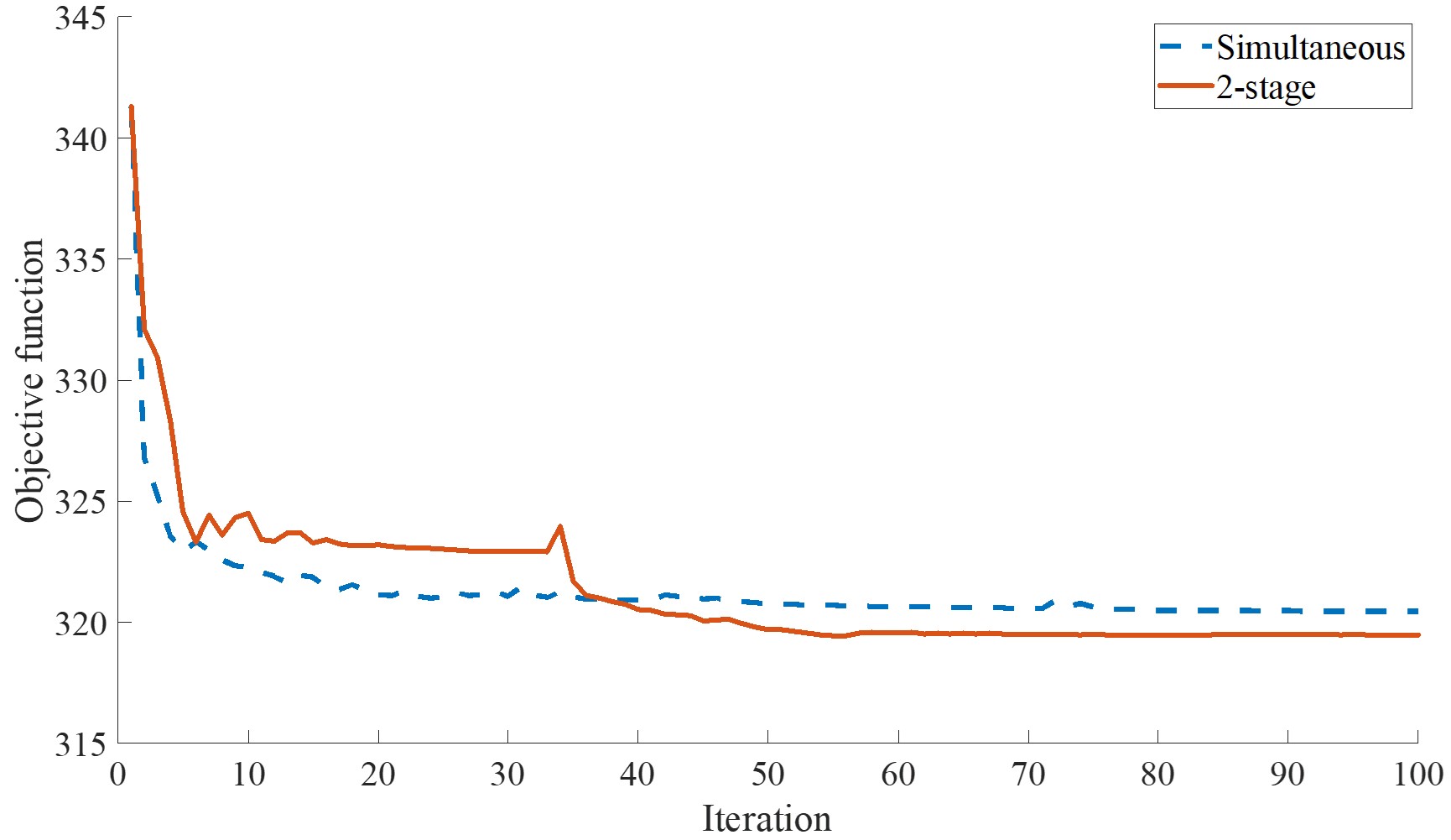
二段階最適化と同時最適化における目的関数履歴の比較
上の目的関数履歴を見ると、同時最適化は壁とフィンを一度に更新するため、最適化の初期段階では目的関数が速く低下しています。
しかし、その後は目的関数の低下が緩やかになり、最終値は約320.46となりました。
一方、二段階最適化は、壁最適化からフィン最適化への切り替えを経て、最終的に約319.48まで低下しています。
両者の目的関数の差は大きくありませんが、二段階最適化では構成要素同士の機能的な競合を抑えながら、同時最適化よりも低い目的関数を得ています。
さらに、得られた形状の物理的な意味が明確であり、大域的な流路を変更する場合は壁のみ、局所的な熱伝達を調整する場合はフィンのみを修正できるため、最適化後の設計調整にも適した結果となっています。
おわりに
本記事では、国際学術誌Structural and Multidisciplinary Optimization (SMO)に採択された研究成果論文について解説しました。
具体的には、冷却流路のトポロジー最適化を対象とし、大域的流路を形成する「壁」と局所的な熱伝達を促進する「フィン」という異なる物理的な役割を割り当てられた構成要素を定義し、役割ごとに最適化段階を分けることで、両者の競合を抑えながら設計できる二段階最適化手法を提案する内容でした。
本研究では固体領域をMMC構成要素で表現しましたが、先行研究[7]に示されるように、流体領域をMMCで表現する手法も選択肢として有効であり、目的や制約に応じた柔軟な拡張が可能です。
提案した最適化フレームワークはあくまで一例であり、実際の設計課題に応じて適切な構成要素および付与する制約・役割を設定し、最適なフレームワークを構築することが重要です。
弊社では、個別の設計課題に応じて最適なフレームワークを構築し、最適化結果を設計者が適切に解釈・活用することで、競争力のある高性能な製品設計を可能にしています。
参考文献
[1] Hirotani, S., Shintani, K., Furusawa, Y., and Yaji, K. ”Topology optimization of cooling channels using dual-type moving morphable components.” Structural and Multidisciplinary Optimization Vol. 69, No. 186, 2026.
[2] Bendsøe, M. P., and Kikuchi, N., “Generating Optimal Topologies in Structural Design Using a Homogenization Method,” Computer Methods in Applied Mechanics and Engineering, Vol. 71, No. 2, 1988, pp. 197–224.
[3] Bendsøe, M. P., “Optimal Shape Design as a Material Distribution Problem,” Structural Optimization, Vol. 1, No. 4, 1989, pp. 193–202.
[4] Guo, X., Zhang, W. S., and Zhong, W. L., “Doing Topology Optimization Explicitly and Geometrically-A New Moving Morphable Components Based Framework,” Journal of Applied Mechanics, Vol. 81, No. 8, 2014, p. 081009.
[5] Hirotani S, Yaji K, Makihara K, and Otsuka K., “Data-driven real-time topology optimization using consistent rotation-based moving morphable components.” AIAA J, Vol. 63, No. 10, 2025, pp. 4491-4497.
[6] Yan, S., Wang, F., Hong, J., and Sigmund, O., “Topology optimization of microchannel heat sinks using a two-layer model.” International Journal of Heat and Mass Transfer, Vol. 143, 2019, 118462.
[7] Yu, M., Ruan, S., Wang, X., Li, Z., and Shen, C., “Topology optimization of thermal-fluid problem using the MMC-based approach,” Structural and Multidisciplinary Optimization, Vol. 60, 2019, pp. 151-165.
A paper co-authored by Shunsuke Hirotani, Kunitaka Shintani, and Yoshikatsu Furusawa of our company, together with Associate Professor Kentaro Yaji of the Graduate School of Engineering, The University of Osaka, has been accepted for publication in the international academic journal Structural and Multidisciplinary Optimization (SMO) [1]. In this article, we aim to provide an accessible explanation of the key ideas and concepts behind the research.
Introduction
Topology optimization can reveal design possibilities that human designers may not readily conceive, making it a powerful tool for developing better-performing products [2].
Among the various topology optimization approaches, density-based topology optimization is widely used and has been applied not only to structural problems but also to thermofluid systems and many other fields [3].
Example of density-based topology optimization applied to a cooling channel
However, topology optimization often produces highly complex geometries, which can make the resulting designs difficult to interpret physically, translate into manufacturable products, and control in terms of manufacturing quality.
Although filters can be used in density-based topology optimization to control member dimensions indirectly, it remains difficult to impose complex design constraints strictly on the optimized geometry.
To obtain practical design solutions based on existing manufacturing technologies, designers must interpret the optimization results and perform post-processing to convert them into manufacturable geometries while taking great care not to compromise optimality.
Post-processing is also essential when converting optimization results into CAD models, because grayscale density distributions must be transformed into clear, well-defined geometries.
In this study, we proposed a topology optimization method for cooling channels that can flexibly incorporate geometric design constraints, such as dimensional limits, while producing results that are physically interpretable and readily adjustable after optimization.
Moving Morphable Components (MMC)
Moving Morphable Components (MMC) is one approach to topology optimization [4].
Conceptual illustration of Moving Morphable Components (MMC)
In the MMC approach, geometric entities that can potentially become members of the optimized design are placed in the design domain as “components,” independently of the finite elements used for analysis. The geometry is then represented through the translation, rotation, enlargement, reduction, and overlap of these components.
For an overview of the MMC formulation and examples applied to structural benchmark problems, please refer to our previous article.
Overview and Comparison of Topology Optimization Methods | Nature Architects Inc.
Because MMC directly treats geometric information, such as component dimensions, positions, and orientations, as design variables, it can strictly incorporate geometric constraints into the optimization problem, including requirements such as:
- “The thickness of this member must remain within a specified range.”
- “This component may move only within a specified region.”
- “Adjacent components must maintain C¹ continuity [5].”
Furthermore, because the design variables are the geometric parameters themselves, the optimized result can be transferred seamlessly to a CAD system, providing an important practical advantage.
Overview of the Proposed Cooling-Channel Optimization Framework
In this study, we defined two types of components with different physical roles: “walls,” which form the global flow-path network, and “fins,” which promote local heat transfer. We then proposed a two-stage optimization method that separates the optimization stages according to these roles, thereby suppressing functional competition between the two component types. The concept of the method is illustrated below.
Conceptual illustration of the proposed two-stage optimization method
- Step 1: Place wall components and fin components within the design domain.
- Step 2: Optimize the global flow-path network using only the wall components as design variables.
- Step 3: Remove wall components whose dimensions fall below a prescribed threshold and that therefore do not contribute to forming the global flow path.
- Step 4: Remove fin components located closer than a prescribed threshold distance to the retained wall components, leaving only the fin candidates used in the second optimization stage.
- Step 5: Optimize the local heat-transfer characteristics within the flow channel using only the retained fin components as design variables.
- Step 6: Finally, remove fin components whose dimensions fall below a prescribed threshold and adopt the resulting structure as the final design.
The detailed optimization procedure consists of Steps 1 through 6 described above.
By separating the optimization stages according to physical roles and pruning components that do not serve the intended function between stages, the method can produce manufacturable results that remain consistent with the designer’s intent.
Thermofluid Analysis Model
This study employs a two-layer thermofluid model consisting of an upper thermofluid layer, which contains the coolant and channel walls, and a lower substrate layer, which receives heat from the heat-generating body [6].
By assuming velocity and temperature distributions in the thickness direction, the inherently three-dimensional flow and heat-transfer problem is reduced to a two-dimensional problem. This enables the large number of analyses required for topology optimization to be performed efficiently.
In the upper thermofluid layer, the fluid is assumed to be incompressible, and the continuity equation is solved:
Here, \(\mathbf{u}\) is the in-plane velocity.
The following momentum conservation equation is used, including a Brinkman resistance term that suppresses flow inside the solid region:
The final term on the right-hand side, \(-\alpha(\gamma)\mathbf{u}\), is the Brinkman resistance.
By assigning a small resistance in the fluid region and a large resistance in the solid region, the flow channel and the channel walls can be represented within the same governing equation.
For the temperature \(T_t\) in the upper thermofluid layer, the model considers heat transport by fluid flow, in-plane thermal conduction, and heat exchange with the lower substrate layer:
The first term represents heat advection by the fluid, the second represents thermal conduction, and the third represents heat transfer between the upper thermofluid layer and the lower substrate layer.
In the lower substrate layer, fluid flow is neglected, and heat conduction within the substrate is calculated using:
Here, \(T_b\) is the representative temperature of the substrate layer, and \(q_0^{\prime\prime}\) is the heat flux supplied by the heat-generating body.
Heat introduced from the heat-generating body into the substrate is conducted through the substrate and then transferred to the fluid or the channel walls in the upper layer.
Mathematical Representation of MMC Components and Their Incorporation into Material Properties
In MMC, walls and fins are represented as explicit geometric components, and their positions, dimensions, and orientations are treated as design variables. In the thermofluid analysis, however, it is necessary to represent whether each location on a fixed finite-element mesh corresponds to fluid or solid using a material distribution field \(\gamma\).
In this study, the shapes of the MMC components are therefore incorporated into the material properties used in the thermofluid analysis through the following sequence:
Here, \(\alpha(\gamma)\) is the flow resistance, \(k_t(\gamma)\) is the effective thermal conductivity of the upper thermofluid layer, and \(h(\gamma)\) is the heat-transfer coefficient between the two layers.
TDF of a Wall Component
Let an arbitrary point in the design domain be \((X,Y)\), and let the center coordinates of a wall component be \((X_0,Y_0)\). First, local coordinates aligned with the orientation of the wall component are defined as follows:
Here, \(s_w\) is the local coordinate along the longitudinal direction of the wall, \(n_w\) is the local coordinate normal to that direction, and \(\theta\) is the rotation angle of the wall component.
The geometry of the wall component is represented by the following sixth-order superelliptic TDF:
Here, \(L\) is the longitudinal dimension, and \(t\) is the transverse dimension.
Using an exponent of six provides a smooth representation of a bar-like wall geometry that is more rectangular than an ordinary ellipse.
TDF of a Fin Component
Similarly, local coordinates are defined for a fin component whose center coordinates are \((X_f,Y_f)\):
Here, \(\psi\) is the rotation angle of the fin.
An elliptical fin component is represented by the following TDF:
\(a\) is the major radius of the ellipse, and \(k\) is the ratio of the minor radius to the major radius. The minor radius \(b\) is therefore:
Thus, the fin is circular when \(k=1\), while decreasing \(k\) produces a more slender ellipse.
Note that \(k\) here denotes the aspect ratio of the fin geometry and is distinct from the thermal conductivities \(k_f\) and \(k_s\) introduced later.
For both wall and fin components, the TDF has the following sign convention:
Conversion from the TDF to the Material Distribution
Because the TDF cannot be used directly as a material distribution ranging from 0 to 1, each TDF is projected approximately onto the interval from 0 to 1 using a hyperbolic tangent function.
The projected TDF of a wall component is:
The projected TDF of a fin component is:
The parameter \(\beta\) controls the sharpness of the transition between fluid and solid at a component boundary. Under this definition, the projected TDF approaches 0 inside a component and 1 outside it.
Rather than multiplying the raw TDFs of the walls and fins directly, the material distribution \(\gamma\) is obtained from the product of these projected functions.
Combined Material Distribution of Walls and Fins
Let \(C_w\) denote the set of wall components and \(C_f\) the set of fin components. The material distribution over the entire design domain is then expressed as:
Here, \(\mathbf{d}_{w,m}\) and \(\mathbf{d}_{f,n}\) are the design variables of the wall and fin components, respectively.
The material distribution in this study is defined by:
Because the projected TDFs are multiplied, if a point lies inside any wall or fin component, the value of \(\gamma\) at that point approaches 0 and the point is treated as solid.
Conversely, at a point outside all components, each projected TDF approaches 1, so \(\gamma\) also approaches 1 and the point is treated as fluid.
Thus, this product represents the union of the solid regions formed by multiple wall and fin components. Regions where walls and fins overlap are also treated as solid.
In the two-stage optimization, only the set of design variables being updated changes; the material-distribution representation itself remains common to both the first and second stages.
Conversion from the Material Distribution to Flow Resistance
The material distribution \(\gamma\) is first incorporated into the Brinkman resistance coefficient \(\alpha(\gamma)\). The resistance between the fluid and solid phases is interpolated using the following RAMP function:
Here, \(\alpha_f\) is the resistance in the fluid region, \(\alpha_s\) is the resistance in the solid region, and \(q_f\) controls the nonlinearity of the interpolation function.
The values at the two endpoints are:
The resistance values on the fluid and solid sides are defined as:
Here, \(\mu\) is the dynamic viscosity of the fluid, and \(H_t\) is the half-thickness of the upper thermofluid layer.
By assigning a much larger resistance to the solid region than to the fluid region, the Brinkman resistance term in the momentum conservation equation,
reduces the velocity inside the walls and fins to nearly zero. In contrast, the resistance is small in the flow-channel region where \(\gamma\simeq1\), allowing the fluid to flow.
Conversion from the Material Distribution to Thermal Conductivity
The material distribution \(\gamma\) is also incorporated into the effective thermal conductivity \(k_t(\gamma)\) of the upper thermofluid layer:
Here, \(k_f\) is the thermal conductivity of the fluid, \(k_s\) is the thermal conductivity of the solid, and \(q_k\) controls the nonlinearity of the interpolation function.
Accordingly, the thermal conductivity of the fluid is used in the flow-channel region, while the thermal conductivity of the solid is used inside the walls and fins.
For intermediate values of \(\gamma\) that appear during optimization, an effective thermal conductivity between the fluid and solid values is assigned.
Conversion from the Material Distribution to the Interlayer Heat-Transfer Coefficient
The heat-transfer coefficient \(h(\gamma)\) between the upper thermofluid layer and the lower substrate layer also depends on the material distribution through the effective thermal conductivity \(k_t(\gamma)\).
The heat-transfer coefficient on the upper thermofluid-layer side is:
The heat-transfer coefficient on the lower substrate-layer side is:
Here, \(k_b\) is the thermal conductivity of the substrate, and \(H_b\) is the half-thickness of the lower substrate layer.
The combined heat-transfer coefficient of the two layers is calculated by treating their thermal resistances as being connected in series:
Consequently, when the shape of an MMC component changes and \(\gamma\) is updated, not only the flow resistance but also the thermal conductivity of the upper layer and the amount of heat transferred from the substrate to the upper layer change.
In summary, a change in the geometry of an MMC component is reflected in the thermofluid analysis through the following sequence:
In other words, when optimization updates the positions, dimensions, and orientations of the walls and fins, their geometries are converted into the material distribution \(\gamma\), and the flow resistance and thermal properties of each finite element are updated accordingly.
This allows geometric changes in the components to be reflected in the flow and temperature fields without remeshing the analysis domain during optimization.
Optimization Problem
Liquid-cooled cold plate considered in the optimization problem
The optimization target is a liquid-cooled cold plate of the type shown above.
The inlet is located at the upper left and the outlet at the lower left. The fluid is driven by prescribing pressure boundary conditions at the inlet and outlet.
Water is used for the material properties of the fluid region, and silicon is used for those of the solid region.
A heat-generating body is modeled by applying a uniform heat flux over the entire design domain.
The objective function is the \(p\)-norm mean of the solid-region temperature shown above. Because \(p=10\) is used, the objective is approximately equivalent to minimizing the maximum temperature.
Optimization Results
Optimized Wall and Fin Configurations at Different Inlet Pressures
In this study, the wall and fin components were optimized under three inlet-pressure conditions: \(P_{in}=50,\ 100,\text{ and }200\ \mathrm{Pa}\).
Optimization of the Wall Components
Optimization result for the wall components at an inlet pressure of 50 Pa
(a) Result for \(P_{in}=50\ \mathrm{Pa}\)
Optimization result for the wall components at an inlet pressure of 100 Pa
(b) Result for \(P_{in}=100\ \mathrm{Pa}\)
Optimization result for the wall components at an inlet pressure of 200 Pa
(c) Result for \(P_{in}=200\ \mathrm{Pa}\)
The figures above show the optimization process for the wall components at each inlet pressure. For each condition, the upper row shows the material distribution, the middle row shows the velocity distribution, and the lower row shows the substrate temperature distribution.
In the initial design, the coolant tends to flow directly from the inlet to the nearby outlet, preventing sufficient flow from reaching the right side of the design domain.
As optimization proceeds, the wall components move and deform so as to block this short-circuit flow under all inlet-pressure conditions, forming a global flow path that redirects the coolant toward the right side of the design domain.
As a result, the coolant passes through a wider portion of the domain, reducing the temperature throughout the substrate.
Objective-function histories during optimization of the wall components
The objective-function histories show a substantial decrease during the early stage of optimization for every inlet pressure, followed by convergence to an almost constant value.
A higher inlet pressure produces a higher flow velocity and therefore stronger convective heat transport, resulting in a lower final objective-function value.
Optimization of the Fin Components
After optimizing the wall components, small wall components that did not contribute to forming the global flow path were removed. The remaining flow-path geometry was then fixed, and the fin components were optimized.
Optimization result for the fin components at an inlet pressure of 50 Pa
(a) Result for \(P_{in}=50\ \mathrm{Pa}\)
Optimization result for the fin components at an inlet pressure of 100 Pa
(b) Result for \(P_{in}=100\ \mathrm{Pa}\)
Optimization result for the fin components at an inlet pressure of 200 Pa
(c) Result for \(P_{in}=200\ \mathrm{Pa}\)
The figures above show that the sizes and orientations of the fins change in response to the local flow, forming geometries that guide the coolant toward high-temperature regions.
At every inlet pressure, optimizing the fins locally adjusts the flow and further improves cooling performance relative to the design obtained by optimizing only the walls.
However, the number and distribution of the fins remaining after optimization depend on the inlet pressure.
At higher inlet pressures, flow turning and recirculation induced by the fins promote fluid mixing and enhance heat transfer by thinning the thermal boundary layer. Consequently, a relatively large number of fins remain.
At lower inlet pressures, convective heat transport is weaker, and the increase in flow resistance caused by the fins becomes relatively more significant. The optimized fins are therefore distributed more sparsely.
Objective-function histories during optimization of the fin components
As shown above, the objective function is further reduced by optimizing the fins.
Comparison with Density-Based Topology Optimization
To evaluate the performance of the proposed method, a comparison was performed with conventional density-based topology optimization under the inlet-pressure condition \(P_{in}=200\ \mathrm{Pa}\).
The thermofluid model, boundary conditions, finite-element mesh, material-property interpolation method, and initial material distribution were identical for the two methods.
Result obtained using density-based topology optimization
Whereas the proposed method uses the positions, dimensions, and orientations of the walls and fins as design variables, the density-based method directly updates density variables assigned to individual finite elements.
The density-based method therefore has very high local geometric freedom, and the result shown above contains many slender features and complex local structures.
Some of the bar-like and elliptical features remaining in the result originate from the initial material distribution shared by both methods; the density-based method itself was not subject to geometric constraints associated with walls or fins.
Comparison of the objective-function histories for the proposed method and the density-based method
The objective-function histories show that, in the proposed method, the objective decreases rapidly during the initial wall-optimization stage, exhibits a temporary variation when the optimization stage is switched, and then decreases further during fin optimization.
In contrast, the density-based method continuously updates all density variables, resulting in a comparatively smooth decrease in the objective function.
The final objective-function values were approximately 319.48 for the proposed method and 319.40 for the density-based method, indicating that the two methods achieved nearly equivalent cooling performance.
The proposed method used 299 design variables, whereas the density-based optimization used 84,480. Thus, the proposed method performed the optimization with approximately 1/283 as many design variables.
Although the local degrees of freedom were greatly reduced by restricting the geometric representation to walls and fins, the proposed method achieved almost the same objective-function value as the density-based method. This result demonstrates the effectiveness of representing the geometry using components whose roles are intentionally defined by the designer.
The important point of this comparison is not that the proposed method generally outperforms the density-based method.
Rather, its significance lies in obtaining a simpler, more interpretable geometry that is easier to modify dimensionally while maintaining cooling performance comparable to that of density-based optimization, despite operating in a more restricted design space.
Comparison with Simultaneous Optimization of Walls and Fins
To examine the effectiveness of the proposed two-stage optimization, it was compared with an approach that simultaneously updates the wall and fin components under the inlet-pressure condition \(P_{in}=200\ \mathrm{Pa}\).
The initial geometry, objective function, governing equations, boundary conditions, material-property interpolation method, and finite-element mesh were identical to those used in the two-stage optimization.
Comparison between the two-stage optimization and simultaneous wall-and-fin optimization
In the simultaneous optimization shown above, all design variables of the walls and fins are updated at the same time.
As a result, some wall components originally introduced to form the global flow path are instead used to promote local heat transfer, while some fin components become involved in forming the global flow path.
The functions of the walls and fins therefore become mixed, making the physical role of each component in the final geometry unclear.
In the two-stage optimization, by contrast, the skeleton of the global flow path is first determined using only the wall components. After that geometry is fixed, only the fin components are used to adjust the local flow and heat transfer.
Consequently, the intended functional division—walls for global flow-path formation and fins for local heat-transfer enhancement—remains clearly visible in the final geometry.
Comparison of the objective-function histories for the two-stage and simultaneous optimization methods
The objective-function histories show that simultaneous optimization reduces the objective rapidly during the early stage because the walls and fins are updated together.
However, the subsequent decrease becomes more gradual, and the final value is approximately 320.46.
The two-stage optimization, in contrast, proceeds from wall optimization to fin optimization and ultimately reaches a value of approximately 319.48.
Although the difference between the two final objective-function values is not large, the two-stage optimization suppresses functional competition between the component types while achieving a lower objective value than simultaneous optimization.
Furthermore, because the physical meaning of the resulting geometry is clear, post-optimization design adjustments can be made by modifying only the walls when changing the global flow path or only the fins when tuning local heat transfer.
Conclusion
This article introduced our research that was accepted for publication in the international journal Structural and Multidisciplinary Optimization (SMO).
The study addressed topology optimization of cooling channels and proposed a two-stage optimization method. Components assigned different physical roles—walls that form the global flow path and fins that promote local heat transfer—are optimized in separate stages to suppress competition between their functions.
Although the solid region was represented using MMC components in this study, representing the fluid region using MMC is also a viable option, as demonstrated in a previous study [7], and the framework can be extended flexibly according to the objective and constraints.
The proposed optimization framework is only one example. For an actual design problem, it is important to select appropriate components, constraints, and physical roles according to the specific requirements and to construct a suitable optimization framework.
At Nature Architects, we develop optimization frameworks tailored to individual design problems and enable the design of competitive, high-performance products by helping designers interpret and utilize optimization results appropriately.
References
[1] Hirotani, S., Shintani, K., Furusawa, Y., and Yaji, K., “Topology optimization of cooling channels using dual-type moving morphable components.” Structural and Multidisciplinary Optimization, Vol. 69, No. 186, 2026.
[2] Bendsøe, M. P., and Kikuchi, N., “Generating Optimal Topologies in Structural Design Using a Homogenization Method,” Computer Methods in Applied Mechanics and Engineering, Vol. 71, No. 2, 1988, pp. 197–224.
[3] Bendsøe, M. P., “Optimal Shape Design as a Material Distribution Problem,” Structural Optimization, Vol. 1, No. 4, 1989, pp. 193–202.
[4] Guo, X., Zhang, W. S., and Zhong, W. L., “Doing Topology Optimization Explicitly and Geometrically—A New Moving Morphable Components Based Framework,” Journal of Applied Mechanics, Vol. 81, No. 8, 2014, p. 081009.
[5] Hirotani, S., Yaji, K., Makihara, K., and Otsuka, K., “Data-driven real-time topology optimization using consistent rotation-based moving morphable components.” AIAA Journal, Vol. 63, No. 10, 2025, pp. 4491–4497.
[6] Yan, S., Wang, F., Hong, J., and Sigmund, O., “Topology optimization of microchannel heat sinks using a two-layer model.” International Journal of Heat and Mass Transfer, Vol. 143, 2019, 118462.
[7] Yu, M., Ruan, S., Wang, X., Li, Z., and Shen, C., “Topology optimization of thermal-fluid problem using the MMC-based approach,” Structural and Multidisciplinary Optimization, Vol. 60, 2019, pp. 151–165.
