
はじめに
本記事は陰関数モデリング(Implicit Modeling)の説明・実演の第2部です。
- 陰関数モデリングに関する説明、TPMS(Triply Periodic Minimal Surface、三重周期極小曲面)によるモデリング
https://nature-architects.com/blog/1115/ - 形状を引数とした陰関数によるモデリング
第2部では形状を引数とした陰関数によるモデリングについて説明と実演を行います。
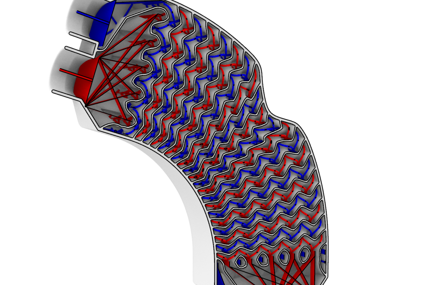
以下のyoutubeの動画で紹介している熱交換構造は、流路の特徴形状から隔壁構造を設計する手法(弊社特許取得済み、特許第7207640号)により陰関数を用いてモデリングをしています。
形状を引数とした陰関数によるモデリング
第1章で示した波状の板の陰関数は、\(k_x,k_y,k_z,\phi_x,\phi_y,t\)を関数を決める引数として持っていました。
\(F(x,y,z|k_x,k_y,k_z,\phi_x,\phi_y,t)=|\cos (k_xx+\phi_x)+\cos (k_yy+\phi_y) +k_zz|-t<0\)
ここでは、\(k_x,k_y,k_z,\phi_x,\phi_y\)はスカラー量でしたが、この引数を形状にして陰関数を定義することもできます。
例えば、形状\(g_1\)を引数として以下のような陰関数による形状表現を考えます。
\(F(x,y,z|g_1,t)=\text{Distance}(p_1,g_1)-t<0
\\
p_1=\text{Point}(x,y,z)\)
\(\text{Point}(x,y,z)\)は\((x,y,z)\)を座標にもつ点、\(\text{Distance}(p_1,g_1)\)は点\(p_1\)と形状\(g_1\)の距離を表す関数と定義すれば、この陰関数表現により形状\(g_1\)に厚さを持たせた構造が生成されます。
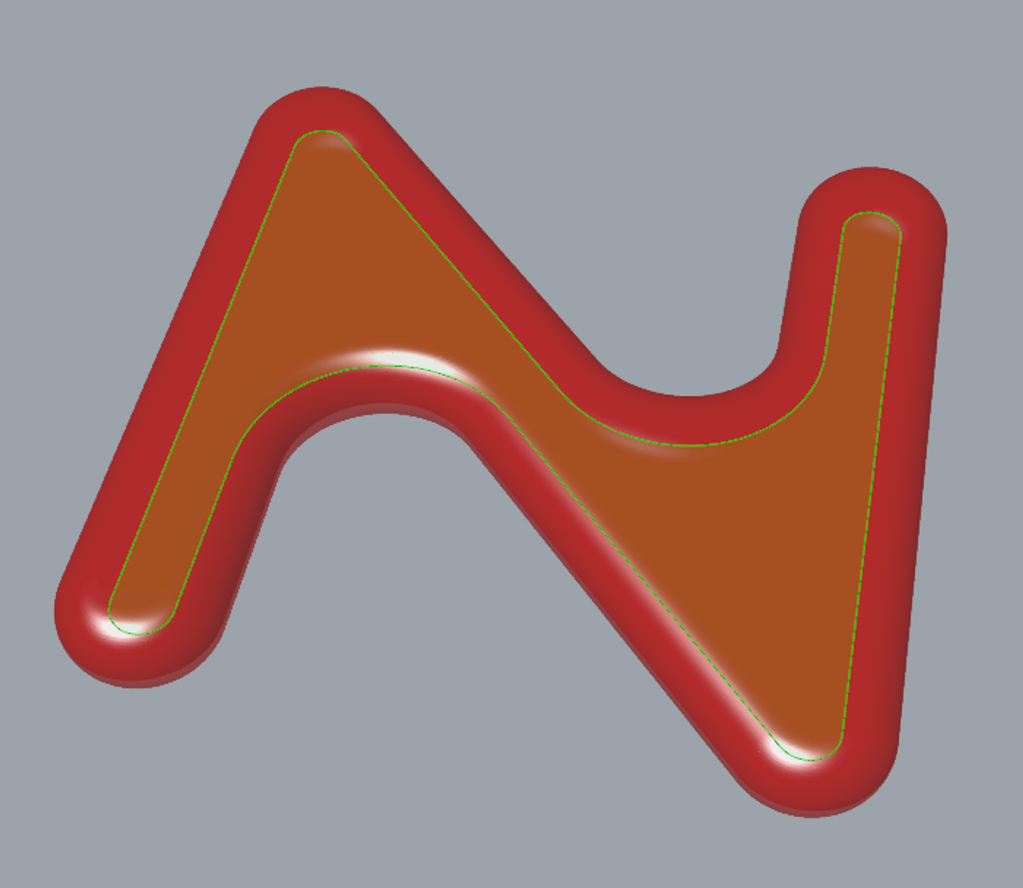
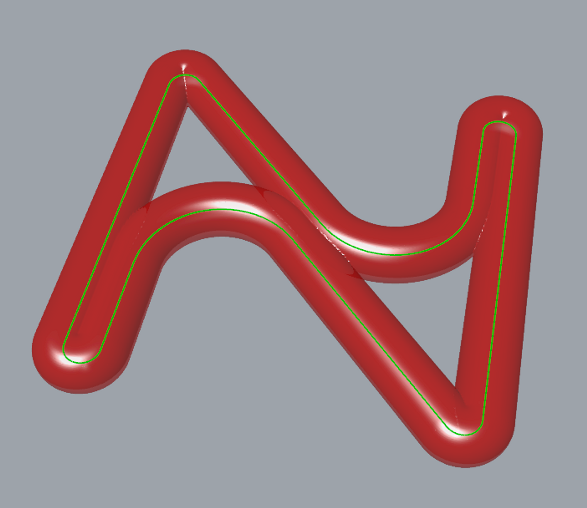
また、第1章の最後にgifで載せていたGyroidにNの形のSchwarz Dを埋め込んだものも、以下のように形状\(g_1\)をもとにした陰関数でモデリングしていました。
\(\begin{aligned}
F(x,y,z|g_1,t)&=|a(x,y,z|g_1)F_{Gyroid}+(1-a(x,y,z|g_1))F_{SchwarzD}+s|-t<0
\\
a(x,y,z|g_1)&=\frac{a_0}{1+\exp(-\alpha d(x,y,z|g_1))}
\\
d(x,y,z|g_1)&=\text{Distance}(p_1,{g_1}_{boundary})\text{sign}(x,y,z|g_1)
\\
p_1&=\text{Point}(x,y,z)
\\
\text{sign}(x,y,z|g_1)&=
\left\{
\begin{matrix}
1 & (\text{if point }(x,y,z) \text{ is contained in } g_1)
\\
-1 &(\text{else})
\end{matrix}
\right.
\end{aligned}\)
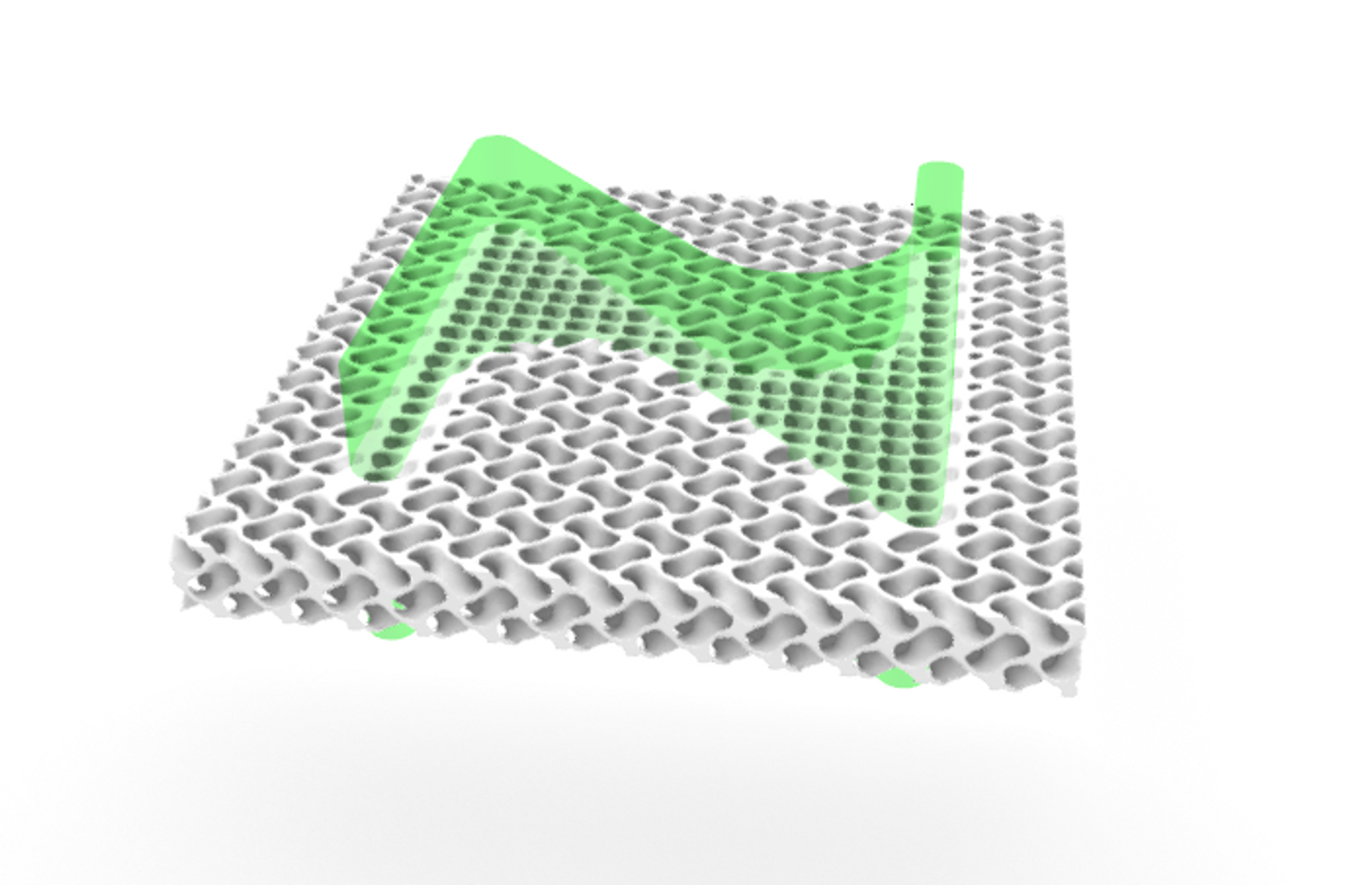
このように形状を引数とした陰関数を用いることで、より複雑なモデリングができます。
ここまでで示した形状を引数とした陰関数は、値の評価に形状と点の距離の見積りを含んでおり、比較的重い演算が必要となります。
そのため複雑な陰関数では構造の生成に時間がかかる可能性があります。
形状をもとにした陰関数モデリングを試してみたい方は、まずは簡単な陰関数を用いて、または構造生成の解像度を落として行うことをおすすめします。
複数の形状を組み合わせた陰関数モデリング
複数の形状を組み合わせた陰関数によりモデリングをすることもできます。
以下の二つに区分された形状の集合\(G_1,G_2\)により定義された陰関数を例にして、実演します。
\(F(x,y,z|G_1,G_2,t)=|\text{Distance}(p_1,G_1)-\text{Distance}(p_1,G_2)+s|-t<0
\\
p_1=\text{Point}(x,y,z)\)
ここで、\(\text{Distance}(p_1,G_1)\)は形状の集合\(G_1\)の中で点\(p_1\)と最も近い形状と\(p_1\)との距離と定義します。
この陰関数は、形状の集合\(G_1,G_2\)の間に隔壁構造を生成するものとなります。
二つの直線によるモデリング
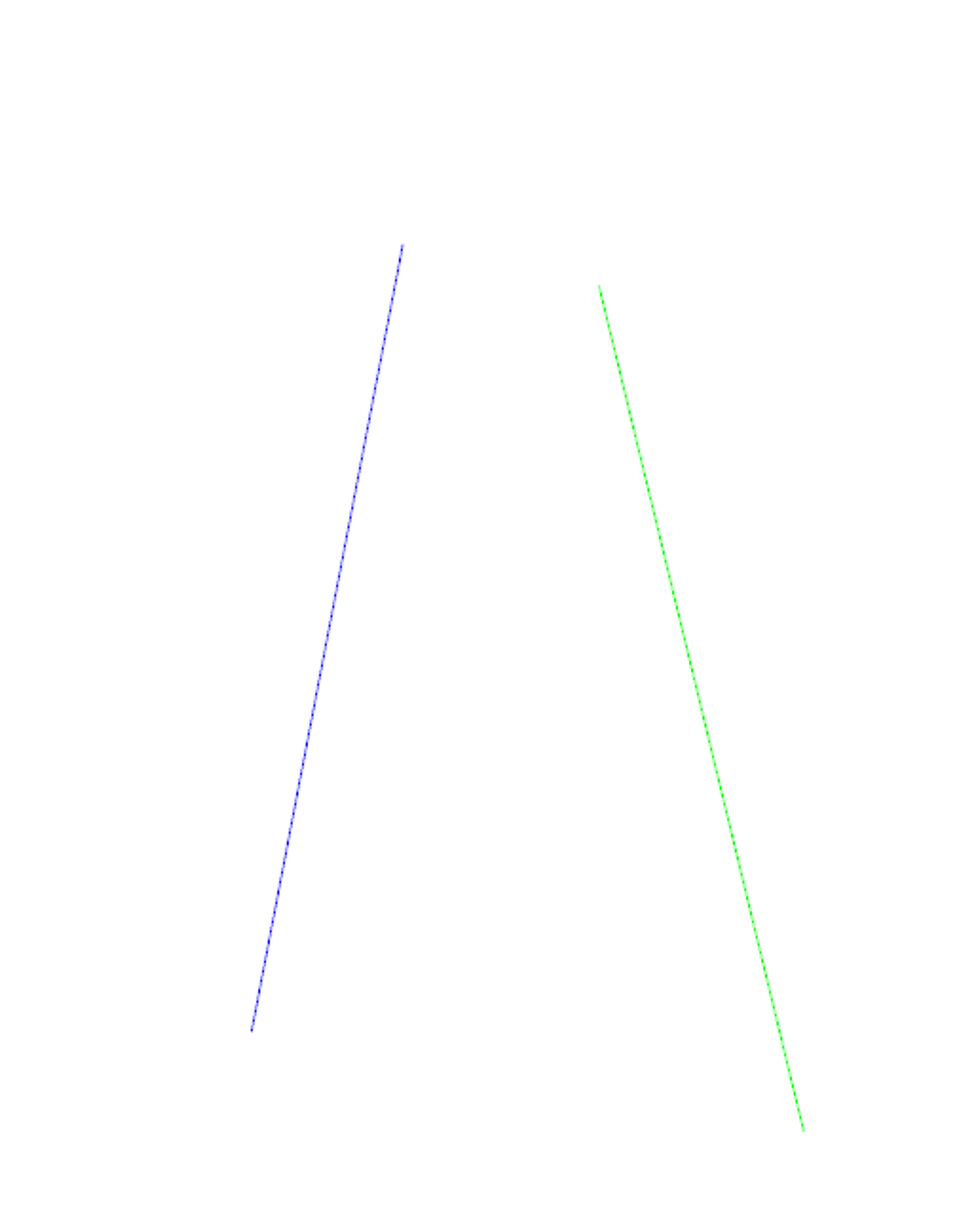
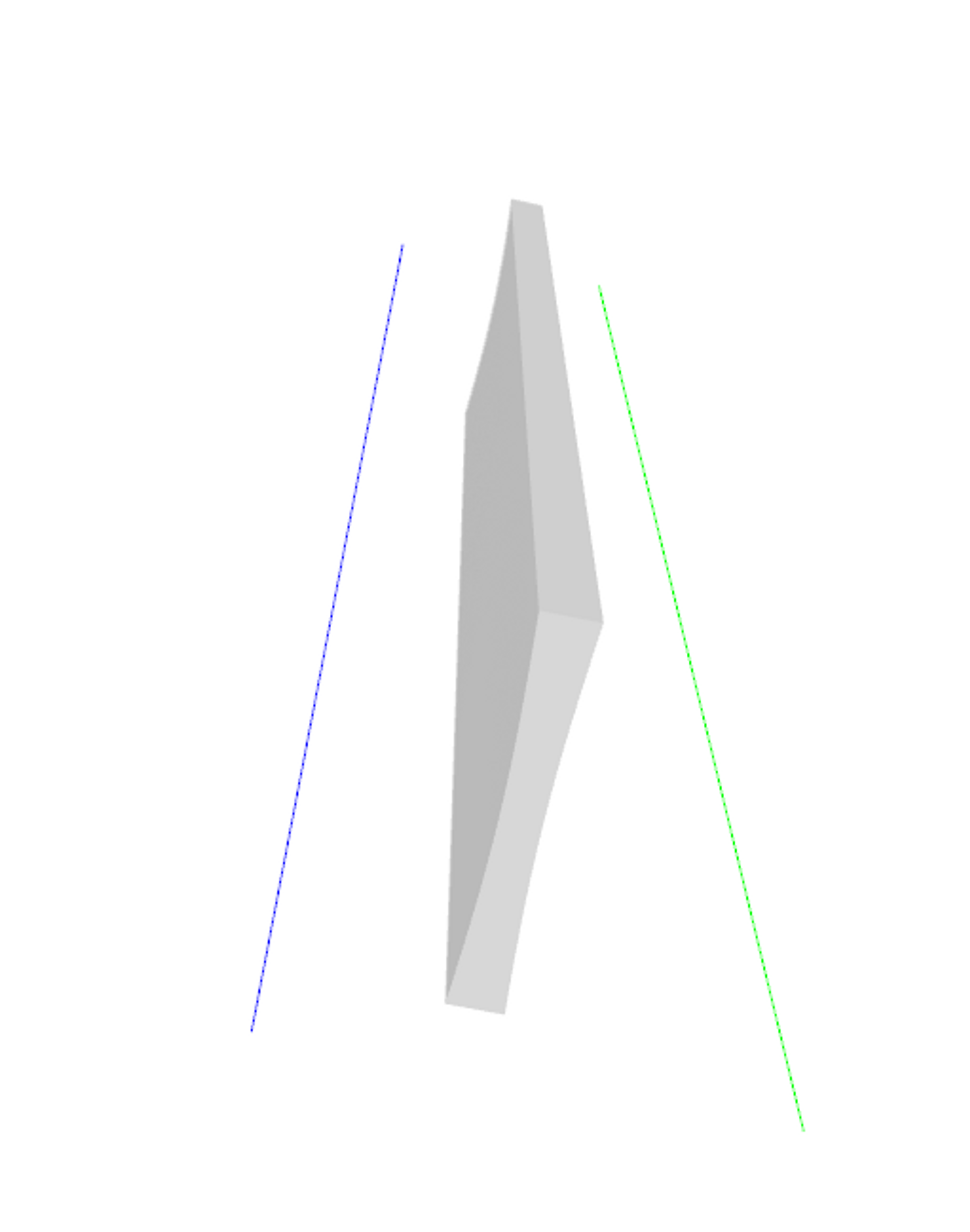
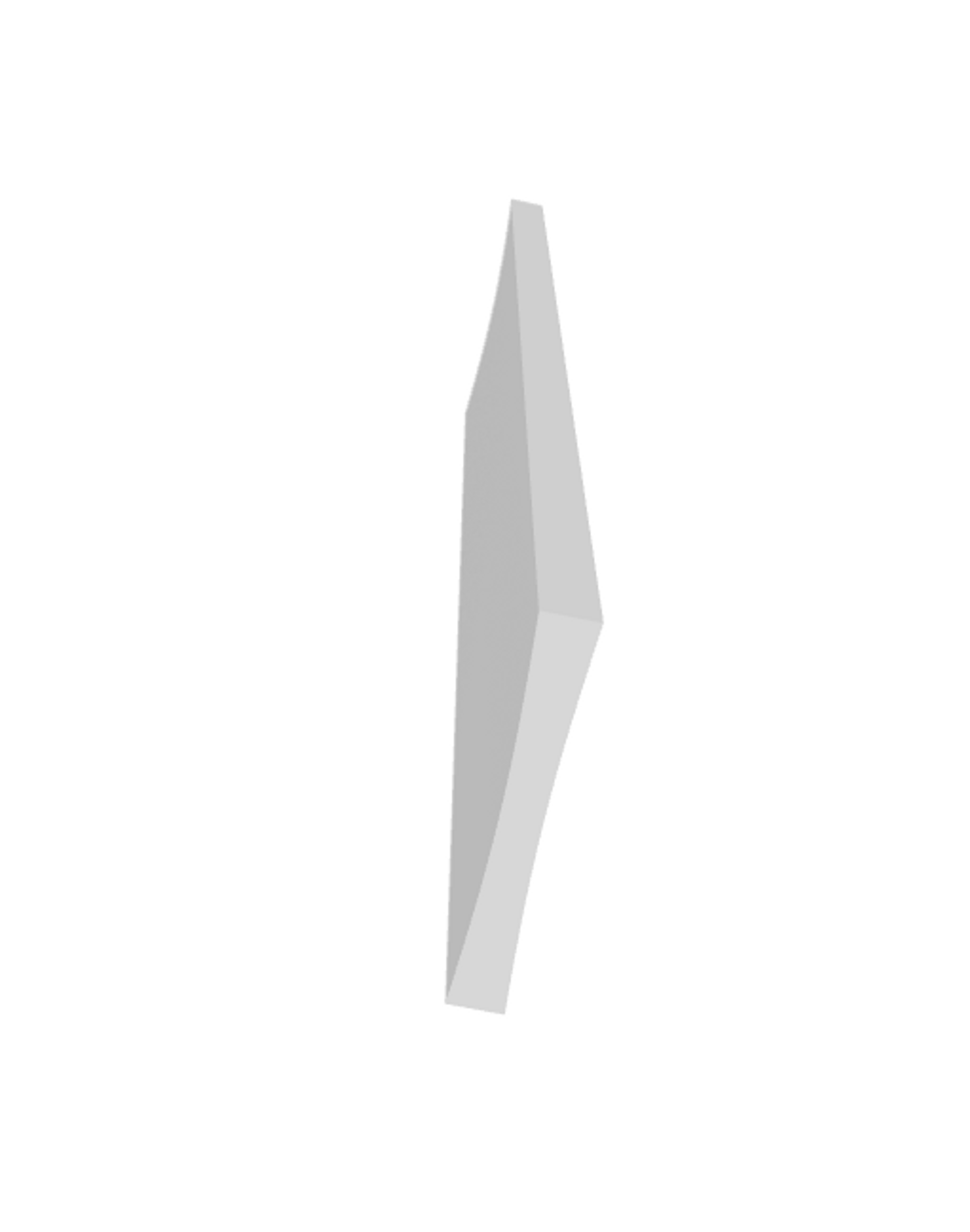
二つの形状を並行な直線で定義すると、直線の間を隔てる構造が生成されます。
\(G_1\):直線(青線)
\(G_2\):直線(緑線)
二つの螺旋によるモデリング
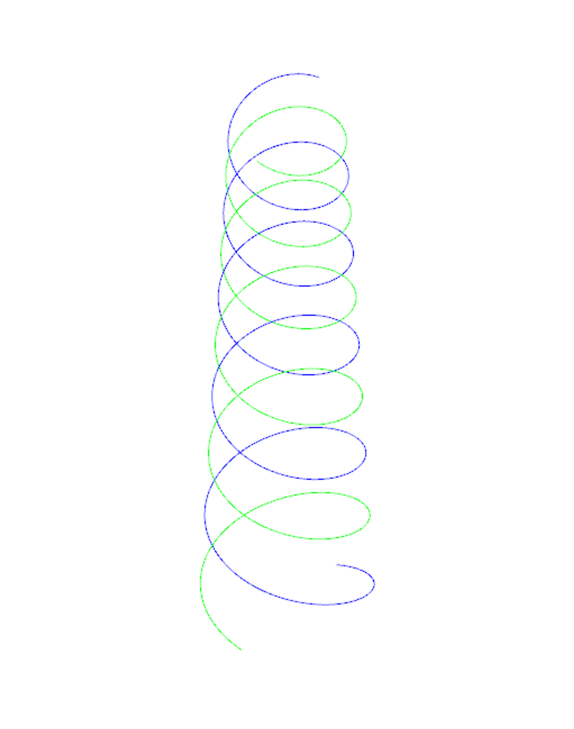
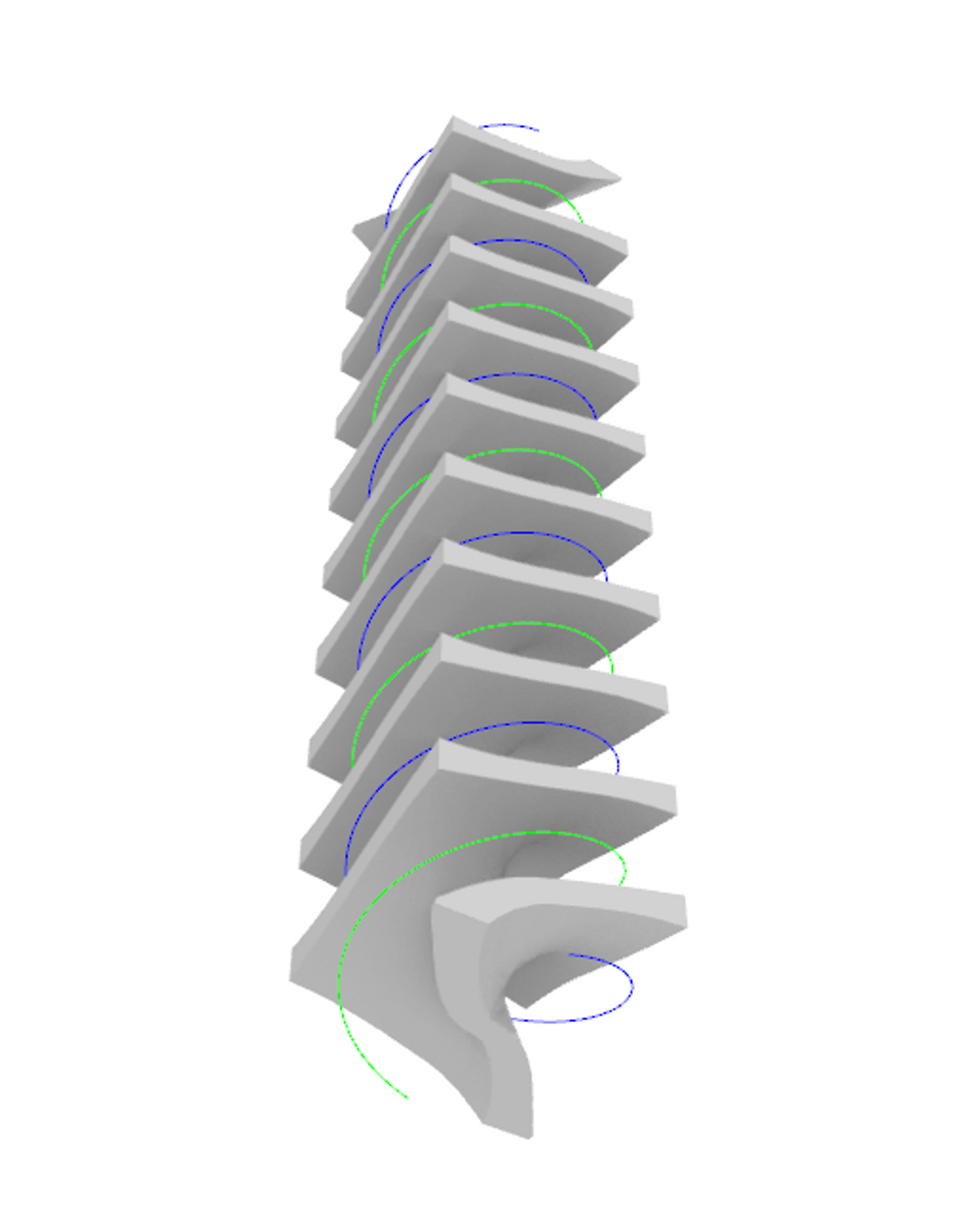
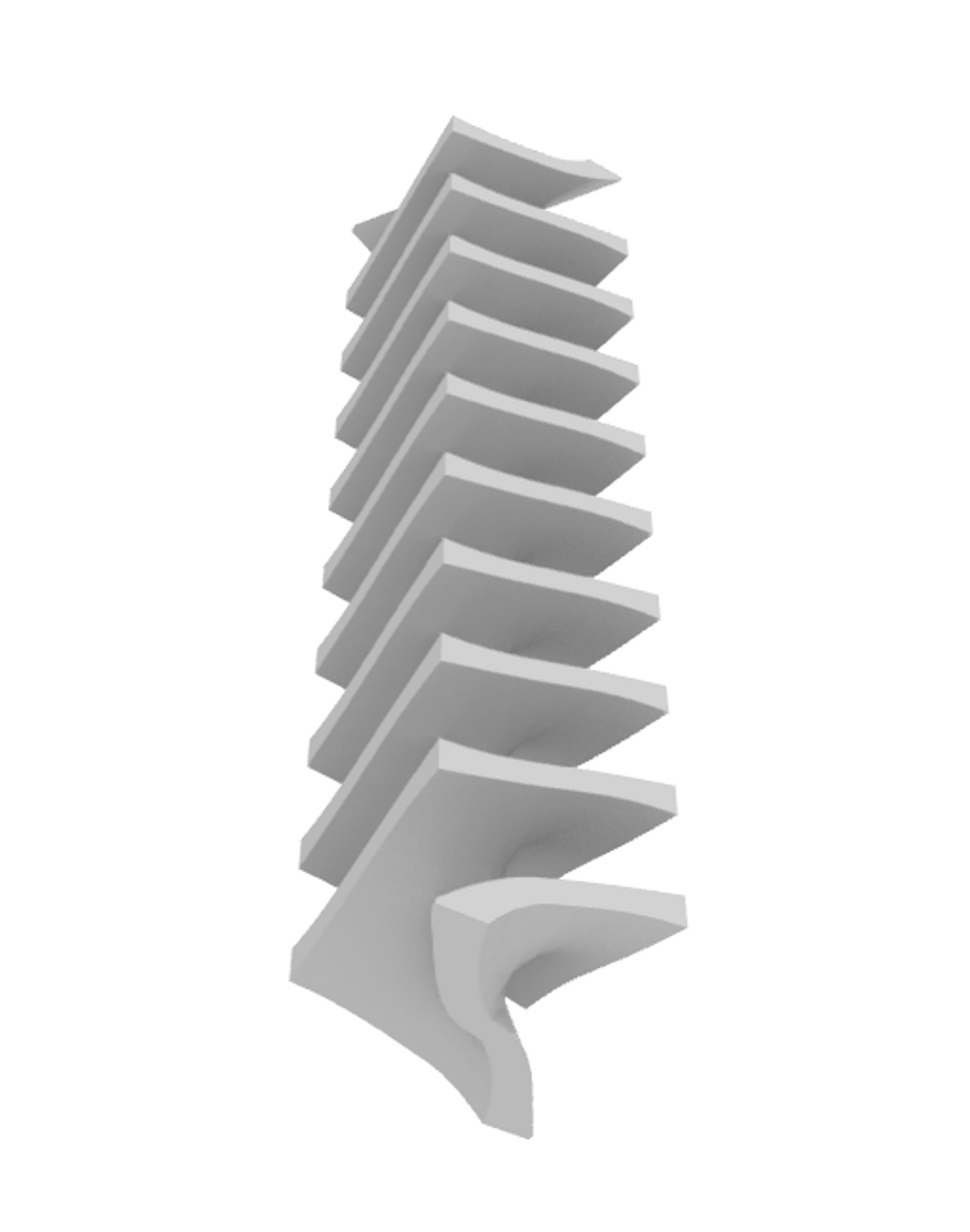
二つの形状を軸が同じで半周期ずれた螺旋で定義すると、螺旋状の隔壁構造が生成されます。
\(G_1\):螺旋(青線)
\(G_2\):螺旋(緑線)
正方格子によるモデリング
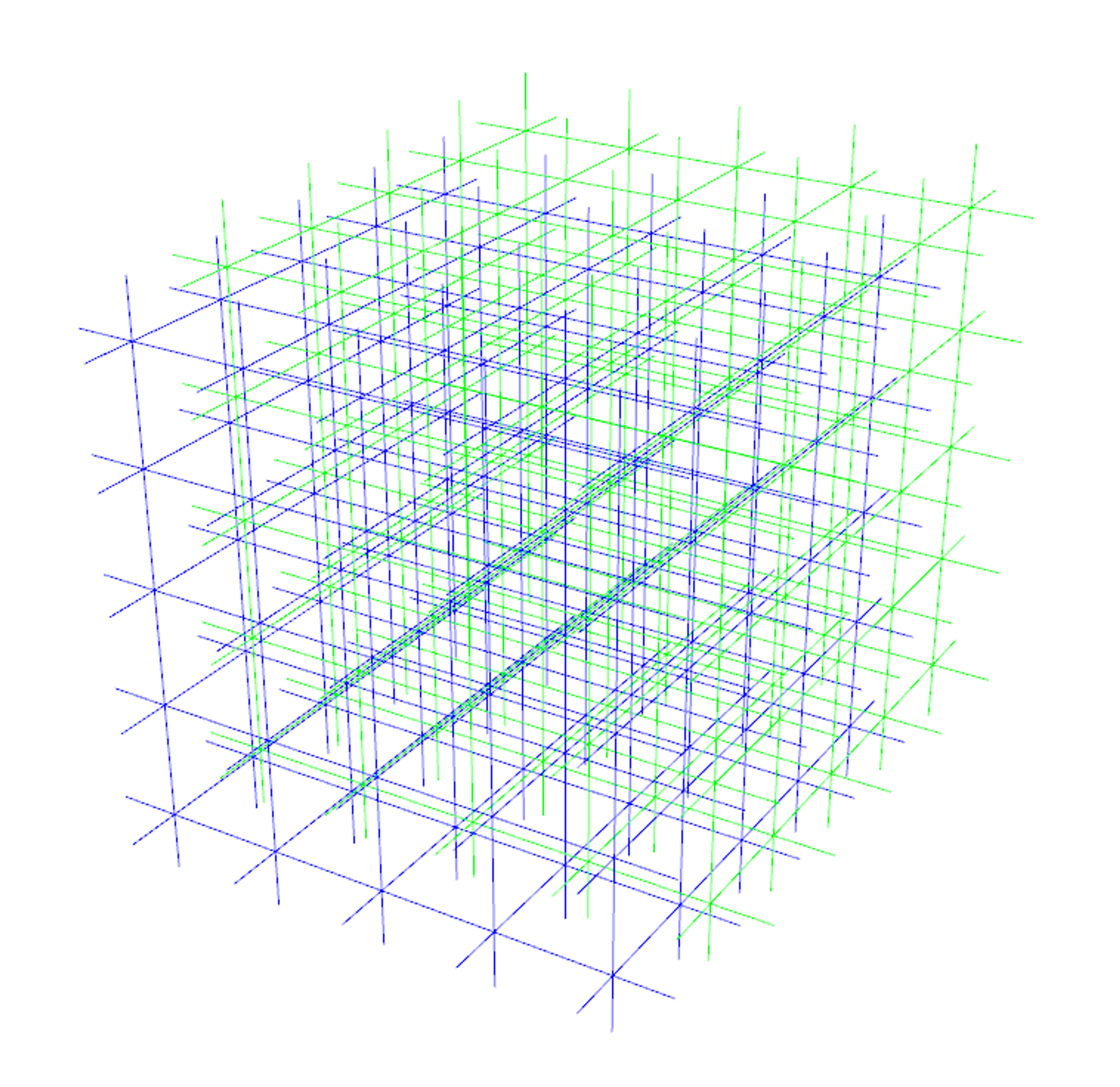
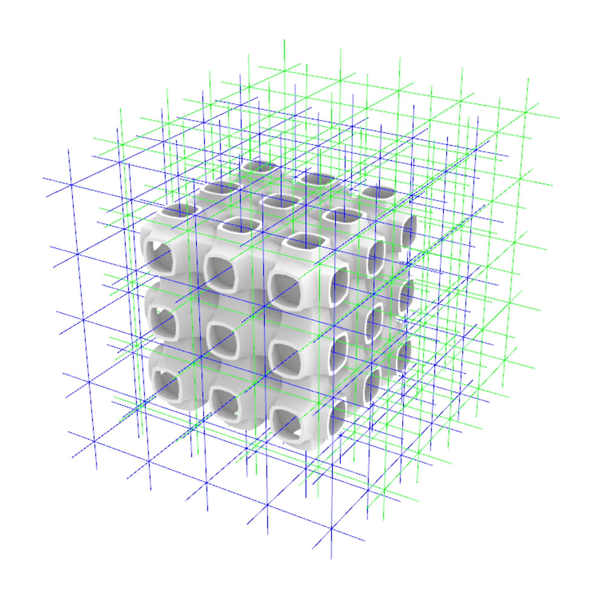
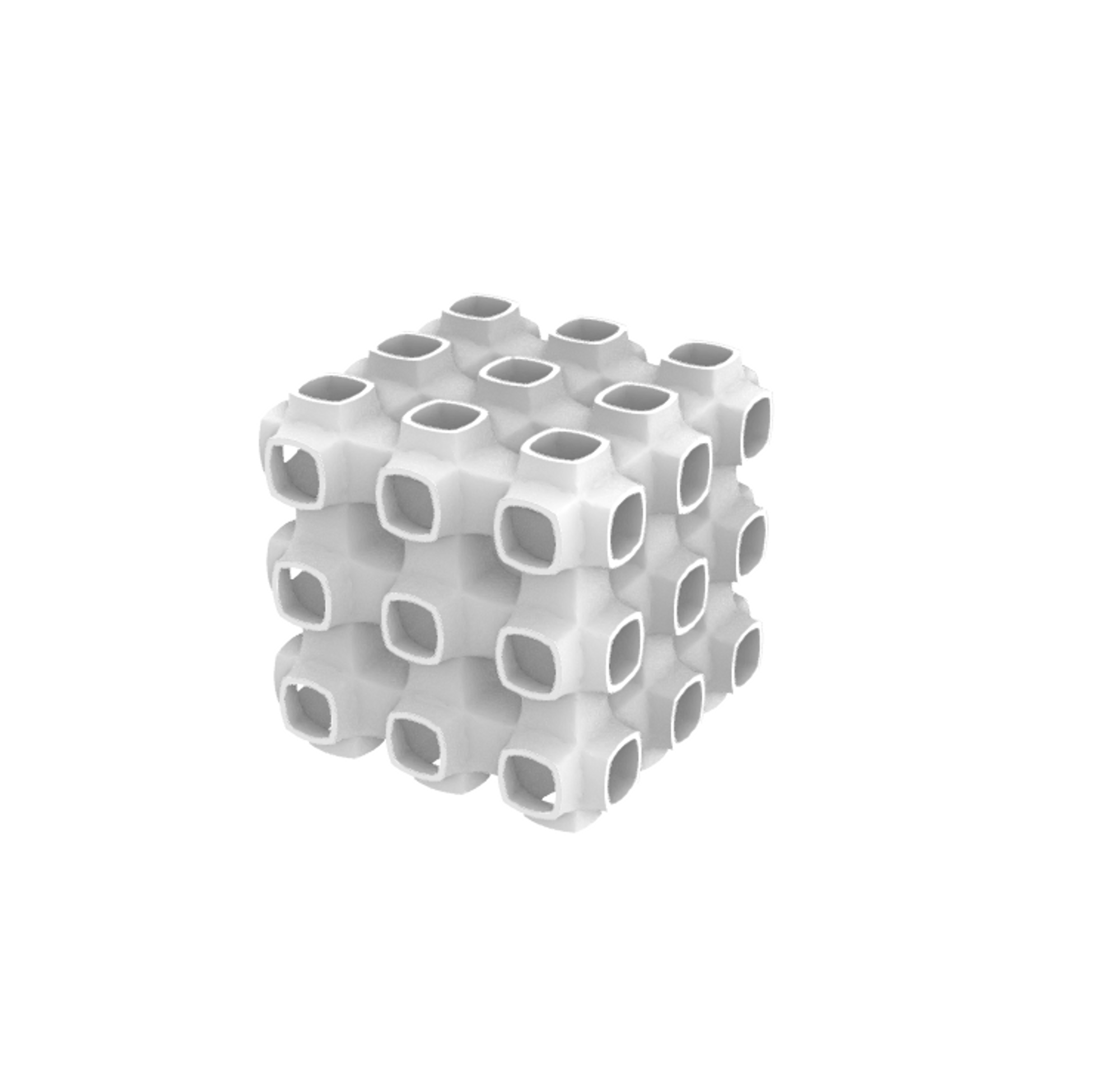
二つの形状の集合を正方格子のスケルトンをもと定義すると、Schwarz Pに似た形状が生成されます。
\(G_1\):正方格子のスケルトン(青線)
\(G_2\):\(G_1\)を各方向に半周期ずらしたもの(緑線)
K4格子によるモデリング
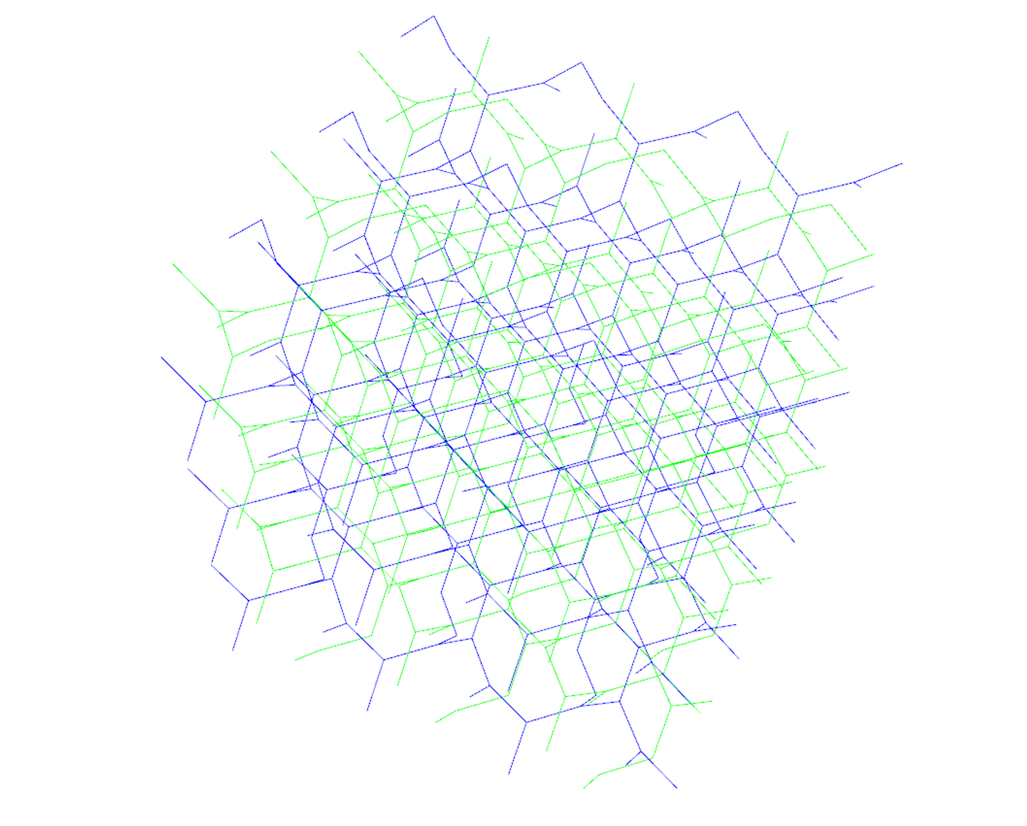
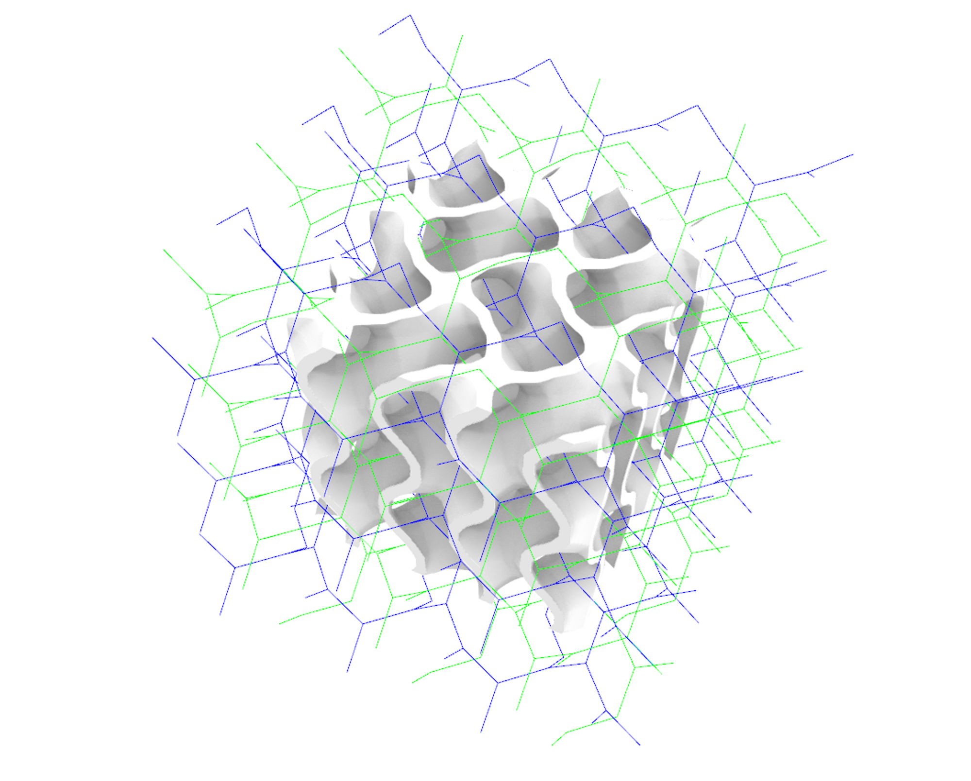
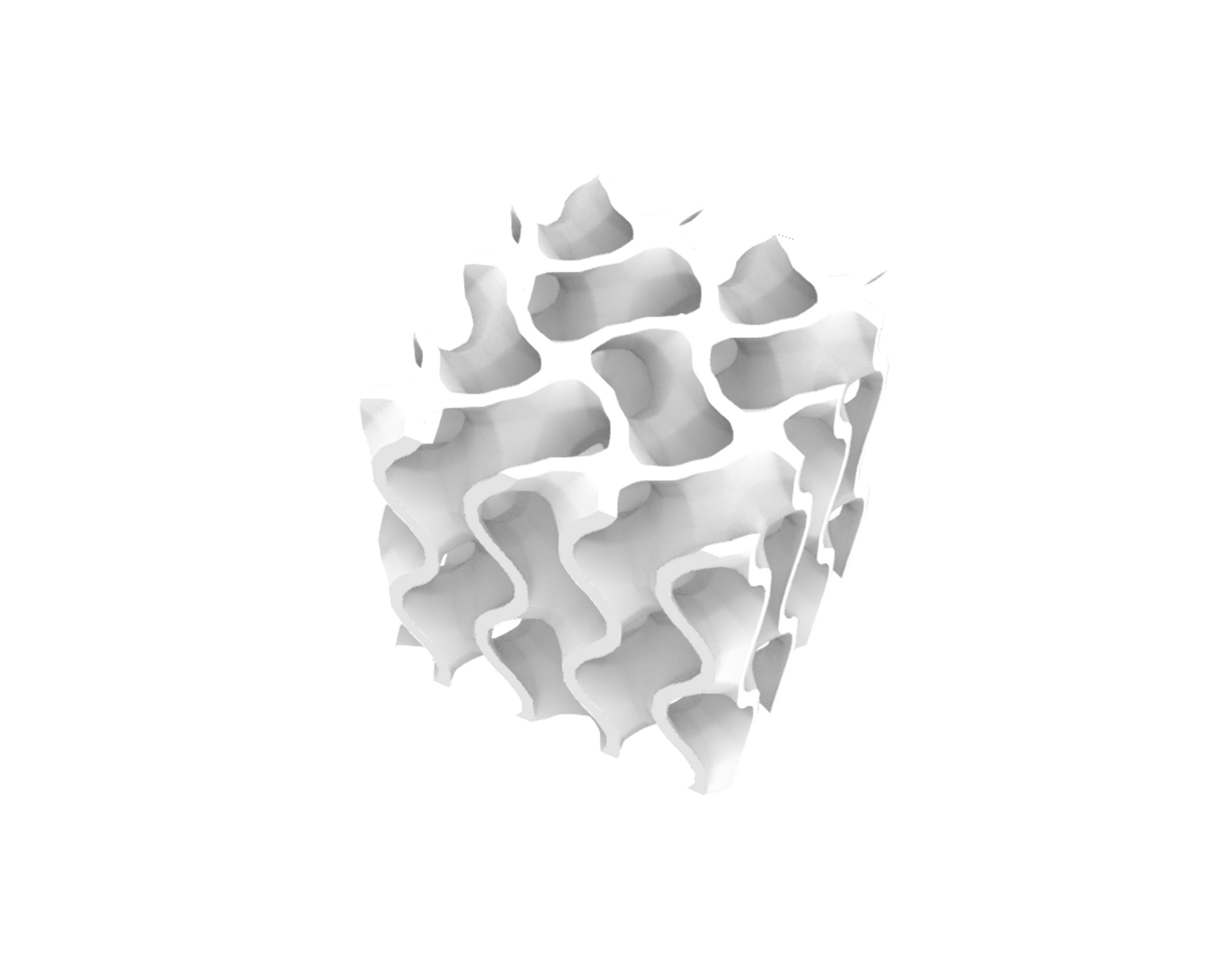
二つの形状の集合をK4格子のスケルトンをもと定義すると、Gyroidに似た形状が生成されます。
\(G_1\):K4格子のスケルトン(青線)
\(G_2\):\(G_1\)を鏡映反転させたもの(緑線)
陰関数による熱交換器のモデリング
「複数の形状を組み合わせた陰関数モデリング」で紹介した陰関数は形状の集合\(G_1,G_2\)の間に隔壁構造を生成するものでした。
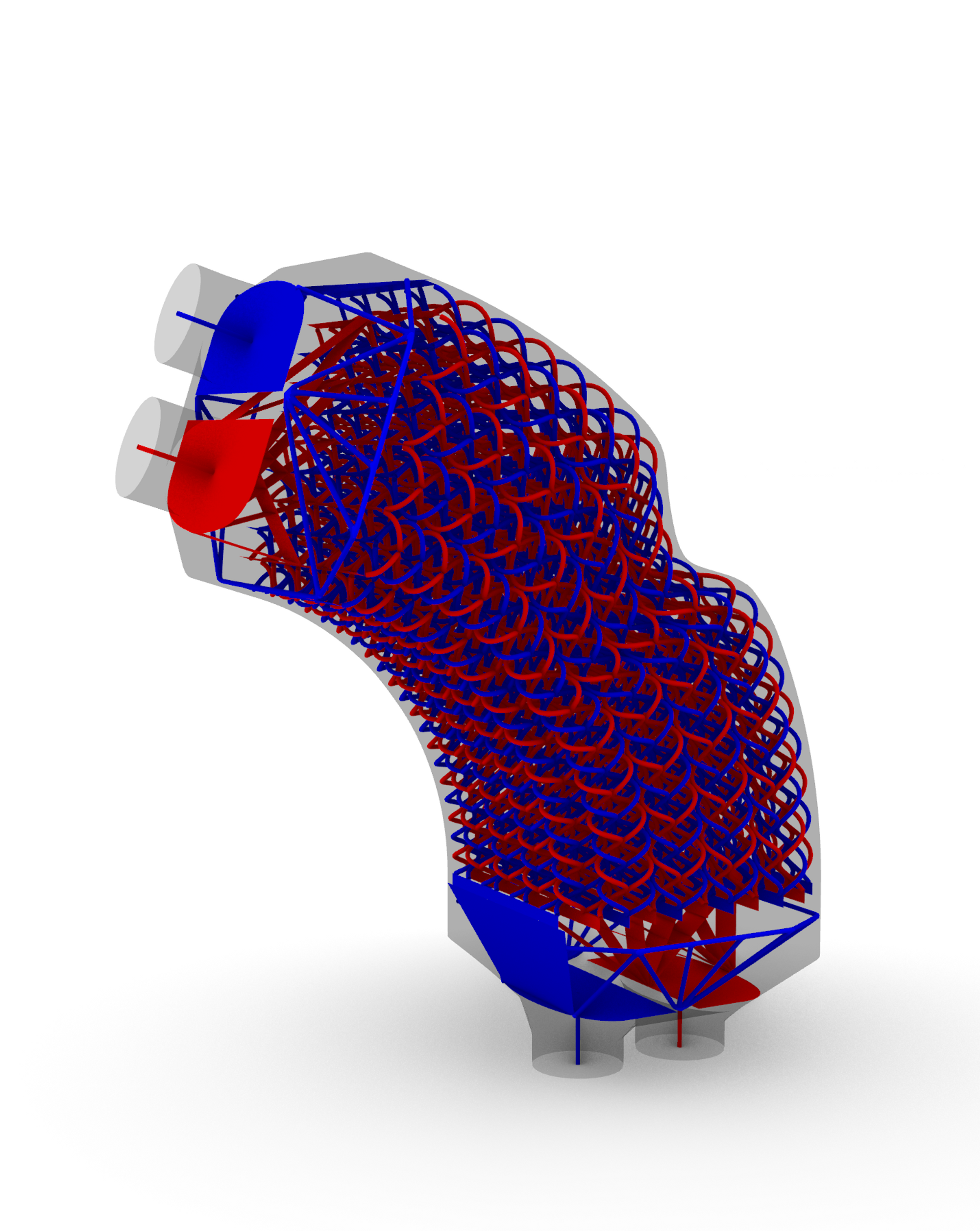
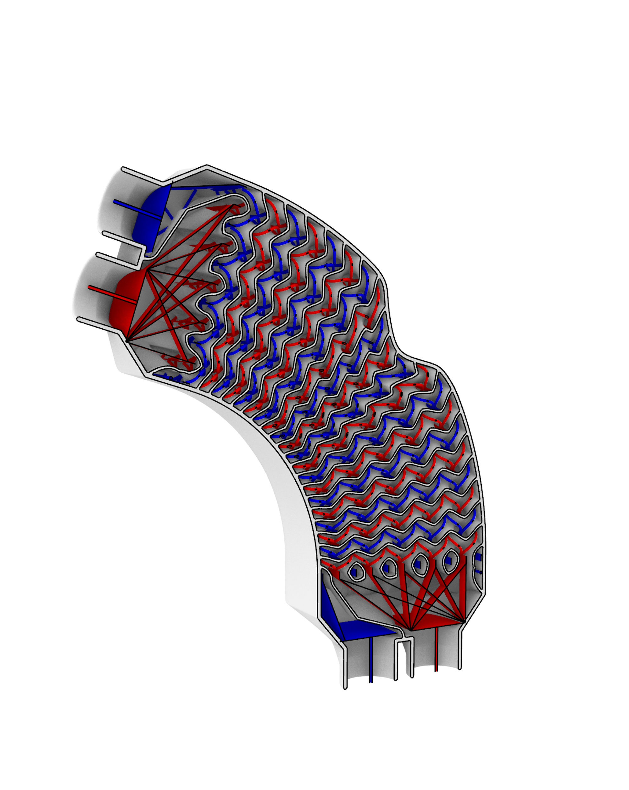
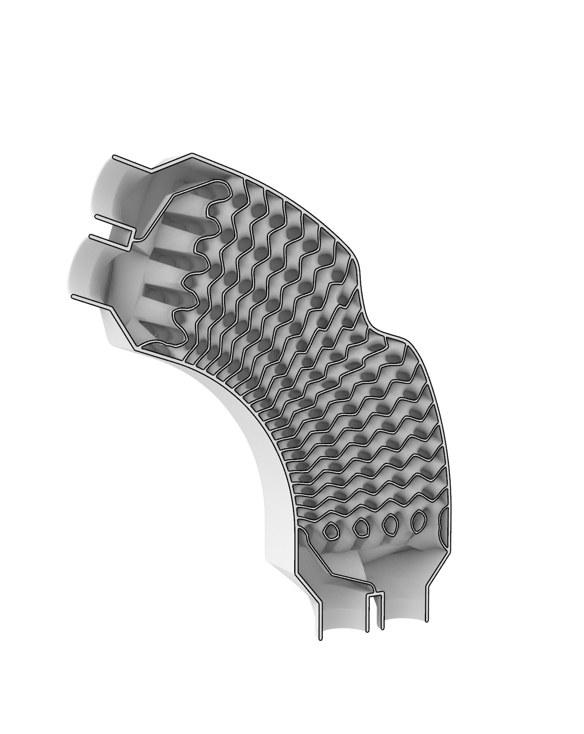
この特徴を利用して、流路の特徴形状として二つの形状の集合を定義すれば、前述した陰関数を用いて2流体の熱交換器(2流体の間で熱を交換する構造)をモデリングすることができます。
実際にモデリングしたものが以下となります。
最後に
第1章では陰関数モデリングの説明とTPMSによるモデリングの実演を、第2章では形状を引数とした陰関数モデリングの説明と実演をしてきました。
陰関数を用いることで数式をもとに複雑なモデリングが可能となり、形状と組み合わせて陰関数を定義することでよりモデリングの幅を広げることができます。
3Dプリント技術の発展により複雑な形状の作成が可能になり、熱交換器をはじめとして産業的にも陰関数を用いたモデリングが利用されています。
本記事を通して、少しでも陰関数モデリングに興味を持ってもらえたらうれしいです。
Introduction
This article is the second part of a explanation and demonstration of Implicit Modeling.
- Explanation of Implicit Modeling, modeling by TPMS (Triply Periodic Minimal Surface)
https://nature-architects.com/blog/1115/ - Implicit modeling with geometry as an argument
In the second part, modeling by implicit functions with geometries as arguments will be explained and demonstrated.
The heat exchange structure shown in the youtube video below is modeled using implicit functions based on our patented method of designing partition structures from the feature geometry of the flow path (our patented method, JP patent No.7207640 ).
Modeling by implicit functions with a geometry as an argument
The implicit function of the corrugated plate shown in Chapter 1 had \(k_x,k_y,k_z,\phi_x,\phi_y,t\) as arguments to determine the function.
\(F(x,y,z|k_x,k_y,k_z,\phi_x,\phi_y,t)=|\cos (k_xx+\phi_x)+\cos (k_yy+\phi_y) +k_zz|-t<0\)
Here, \(k_x,k_y,k_z,\phi_x,\phi_y\) were scalar quantities, but you can also define an implicit function with this argument as the geometries.
For example, consider the following implicit function representation with the geometry \(g_1\) as an argument.
\(F(x,y,z|g_1,t)=\text{Distance}(p_1,g_1)-t<0
\\
p_1=\text{Point}(x,y,z)\)
If we define \(\text{Point}(x,y,z)\) as a point with coordinates `(x,y,z)$ and \(\text{Distance}(p_1,g_1)\) as a function representing the distance between point \(p_1\) and geometry \(g_1\), this implicit function expression generates a structure with thickness in the geometry \(g_1\).
Also, the Schwarz D embedded in Gyroid with the shape of N, which I had put in a gif at the end of Chapter 1, was also modeled with an implicit function based on the geometry \(g_1\) as follows.
\(\begin{aligned}
F(x,y,z|g_1,t)&=|a(x,y,z|g_1)F_{Gyroid}+(1-a(x,y,z|g_1))F_{Diamond}+s|-t<0
\\
a(x,y,z|g_1)&=\frac{a_0}{1+\exp(-\alpha d(x,y,z|g_1))}
\\
d(x,y,z|g_1)&=\text{Distance}(p_1,{g_1}_{boundary})\text{sign}(x,y,z|g_1)
\\
p_1&=\text{Point}(x,y,z)
\\
\text{sign}(x,y,z|g_1)&=
\left\{
\begin{matrix}
1 & (\text{if point }(x,y,z) \text{ is contained in } g_1)
\\
-1 &(\text{else})
\end{matrix}
\right.
\end{aligned}\)
Thus, more complex modeling can be done by using implicit functions with geometries as arguments.
The implicit functions with a geometry as an argument shown so far involve relatively heavy calculation, as the evaluation of the value involves estimating the distance between the geometry and the point.
Therefore, complex implicit functions can take a long time to generate structures.
If you would like to experiment with geometry-based implicit function modeling, we recommend that you start with simple implicit functions or with reduced resolution for structure generation.
Implicit function modeling combining multiple geometries
We can also model by implicit functions that combine multiple geometries.
We will demonstrate with the example of an implicit function defined by the following set of two classified geometries \(G_1,G_2\).
\(F(x,y,z|G_1,G_2,t)=|\text{Distance}(p_1,G_1)-\text{Distance}(p_1,G_2)+s|-t<0
\\
p_1=\text{Point}(x,y,z)\)
Here, \(\text{Distance}(p_1,G_1)\) is defined as the distance between point \(p_1\) and the nearest geometry to \(p_1\) in the set of geometries \(G_1\).
This implicit function will generate a partition structure between the sets of geometries \(G_1,G_2\).
Modeling with two straight lines
Defining two geometries with parallel straight lines generates a structure that separates the lines.
\(G_1\) : one straight line (blue line)
\(G_2\) : one straight line (green line)
Modeling with two spirals
Defining the two geometries as a spiral with the same axis and a half-period shift generates a spiral septum structure.
\(G_1\) : one spiral (blue line)
\(G_2\) : one spiral (green line)
Modeling with square lattice
Defining two sets of geometries based on the skeleton of a square lattice generates a geometry similar to Schwarz P.
\(G_1\) : Square lattice skeleton (blue line)
\(G_2\) : \(G_1\) shifted by half a period in each direction (green line)
Modeling with K4 lattice
Defining two sets of geometries based on the skeleton of the K4 lattice generates a geometry similar to Gyroid.
\(G_1\) : Skeleton of K4 lattice (blue line)
\(G_2\) : Mirror reversal of \(G_1\) (green line)
Modeling of heat exchanger with implicit function
The implicit function introduced in "Implicit function modeling combining multiple geometries" was to generate a partition structure between the sets of geometries \(G_1, G_2\).
Using this feature, a two-fluid heat exchanger (a structure that exchanges heat between two fluids) can be modeled using the aforementioned implicit function by defining two sets of geometries as the feature geometry of the flow path.
The actual modeling is shown below.
Conclusion
In Chapter 1, we have explained implicit modeling and demonstrated modeling with TPMS, and in Chapter 2, we have explained and demonstrated implicit modeling with geometries as arguments.
Implicit functions allow for complex modeling based on mathematical formulas, and defining implicit functions in combination with geometry allows for a wider range of modeling.
The development of 3D printing technology has made it possible to create complex shapes, and modeling with implicit functions is being used industrially, including in heat exchangers.
We hope that through this article, you have gained some interest in implicit function modeling.
