
はじめに
本記事では以下の2部構成で、陰関数モデリング(Implicit Modeling)の説明・実演をしていきます。
- 陰関数モデリングに関する説明、TPMS(Triply Periodic Minimal Surface、三重周期極小曲面)によるモデリング
- 形状を引数とした陰関数によるモデリング
モデリングには主にRhinoceros-GrasshopperのプラグインJellyfishを使用しています。
第1章では陰関数モデリングの説明と、TPMSによる様々なモデリングを行っていきます。
陰関数モデリングとは?
\(y = f(x)\)のように変数の一方について解かれた形式の関数は陽関数と呼ばれます。一方、\(F(x, y) = 0\)のように解けた形式で書かれていない関数は陰関数と呼ばれます。陰関数モデリングは陰関数による表現で形状をモデリングする手法です。
例えば円をモデリングするときは、以下のように陰関数を定義します。
\(F(x,y)=x^2+y^2-R^2\)
この陰関数をもとにした等式または不等式で領域を定義してモデリングを行います。
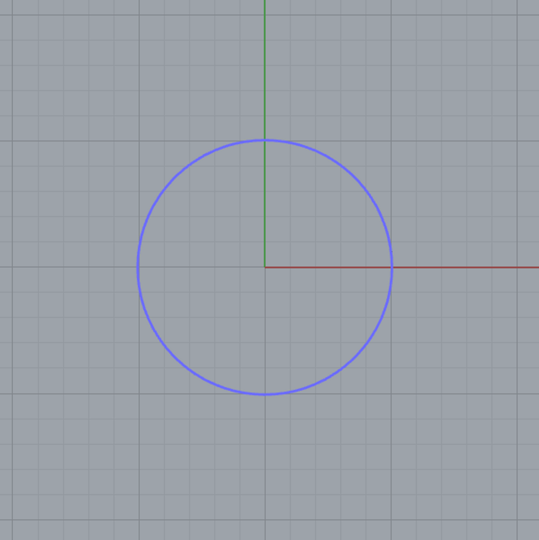
例えば上記陰関数において\(R=5\)として、\(F(x,y)=0\)の領域に形状を生成すると\(xy\)平面に以下のような円が生成されます。(可視化の都合上、円に厚さを持たせています)
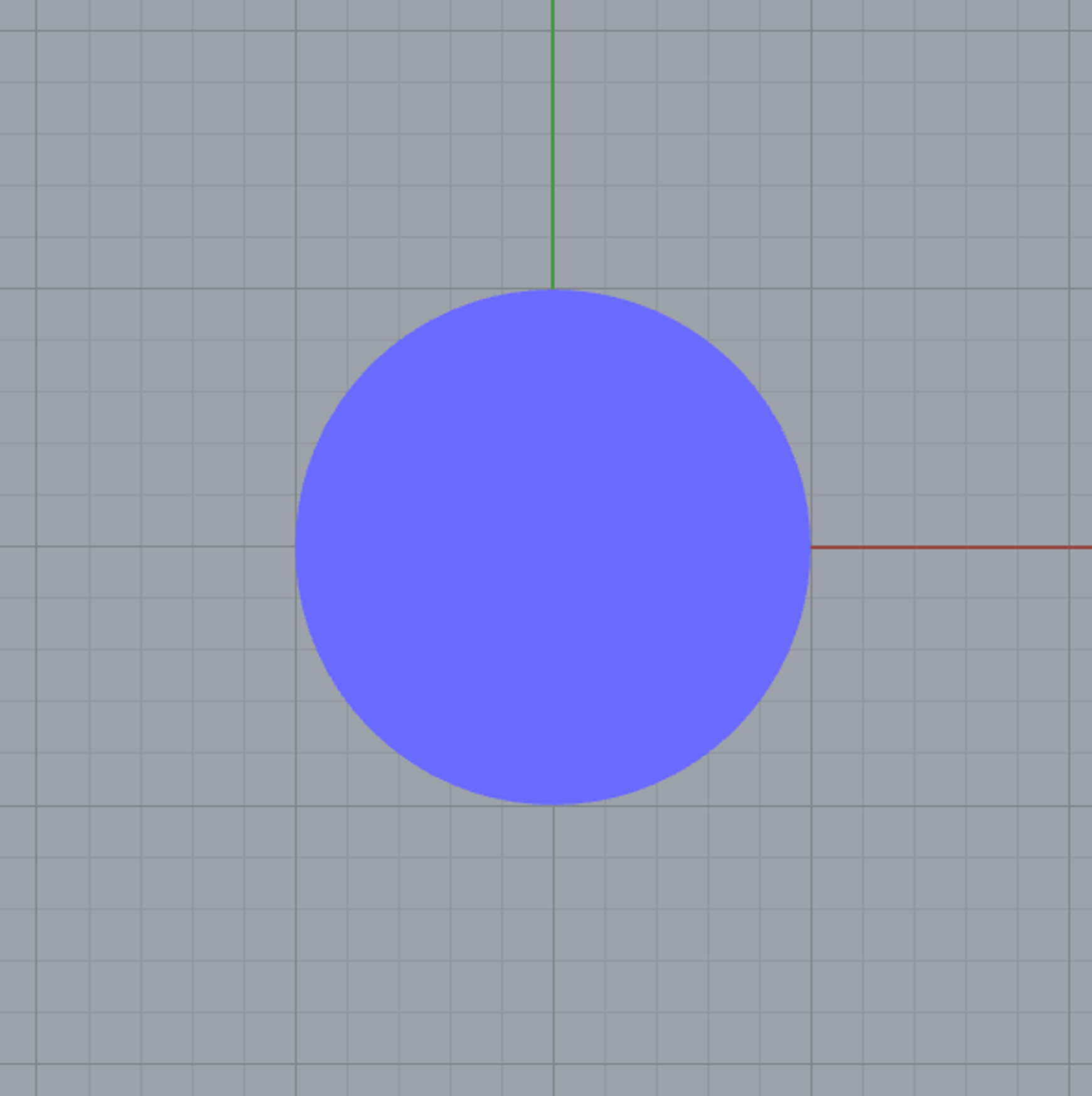
\(F(x,y)\leq 0\)とすれば内部が充填された円となります。
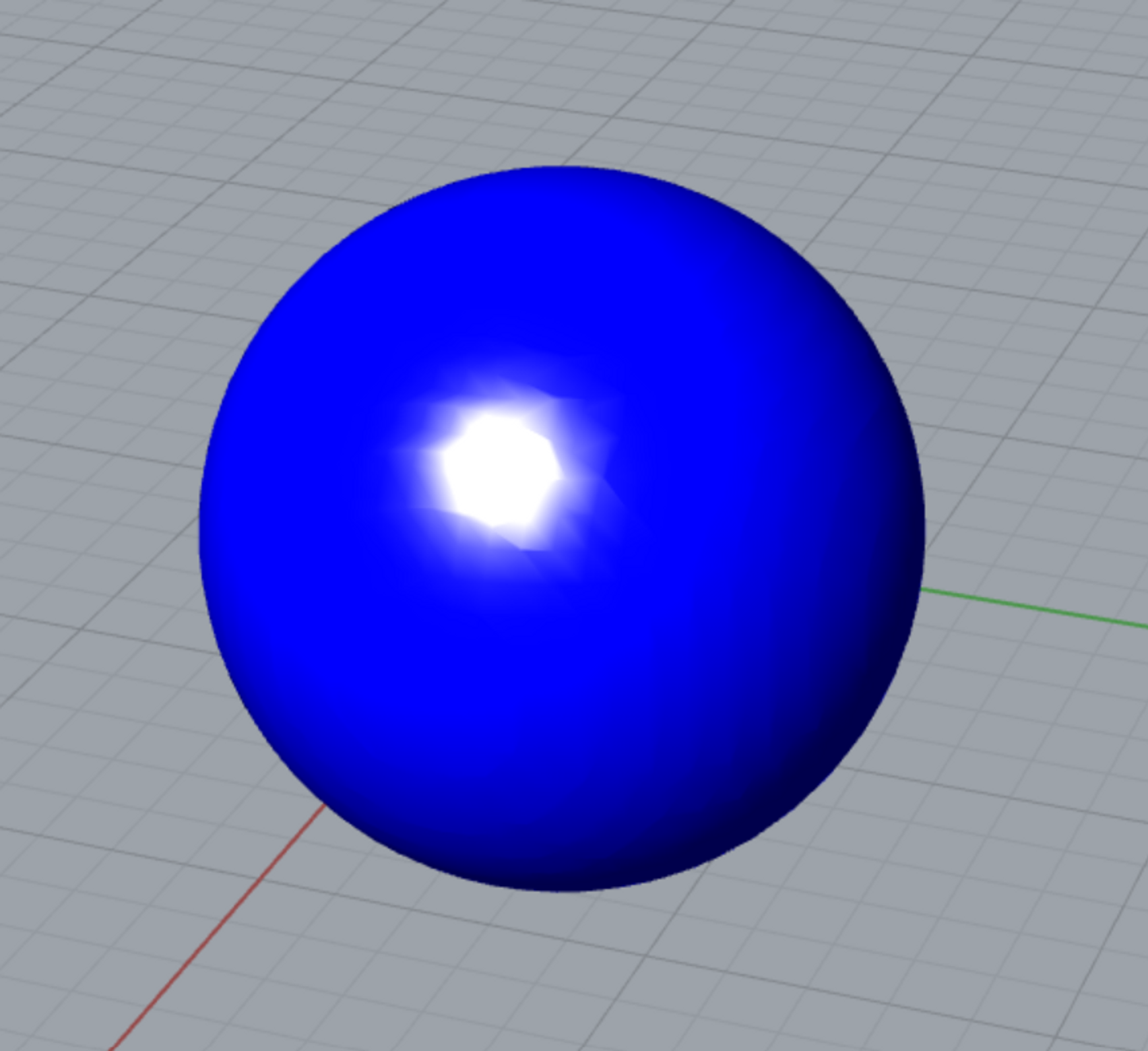
\(F(x,y,z)=x^2+y^2+z^2-R^2< 0\)とすれば球となります。
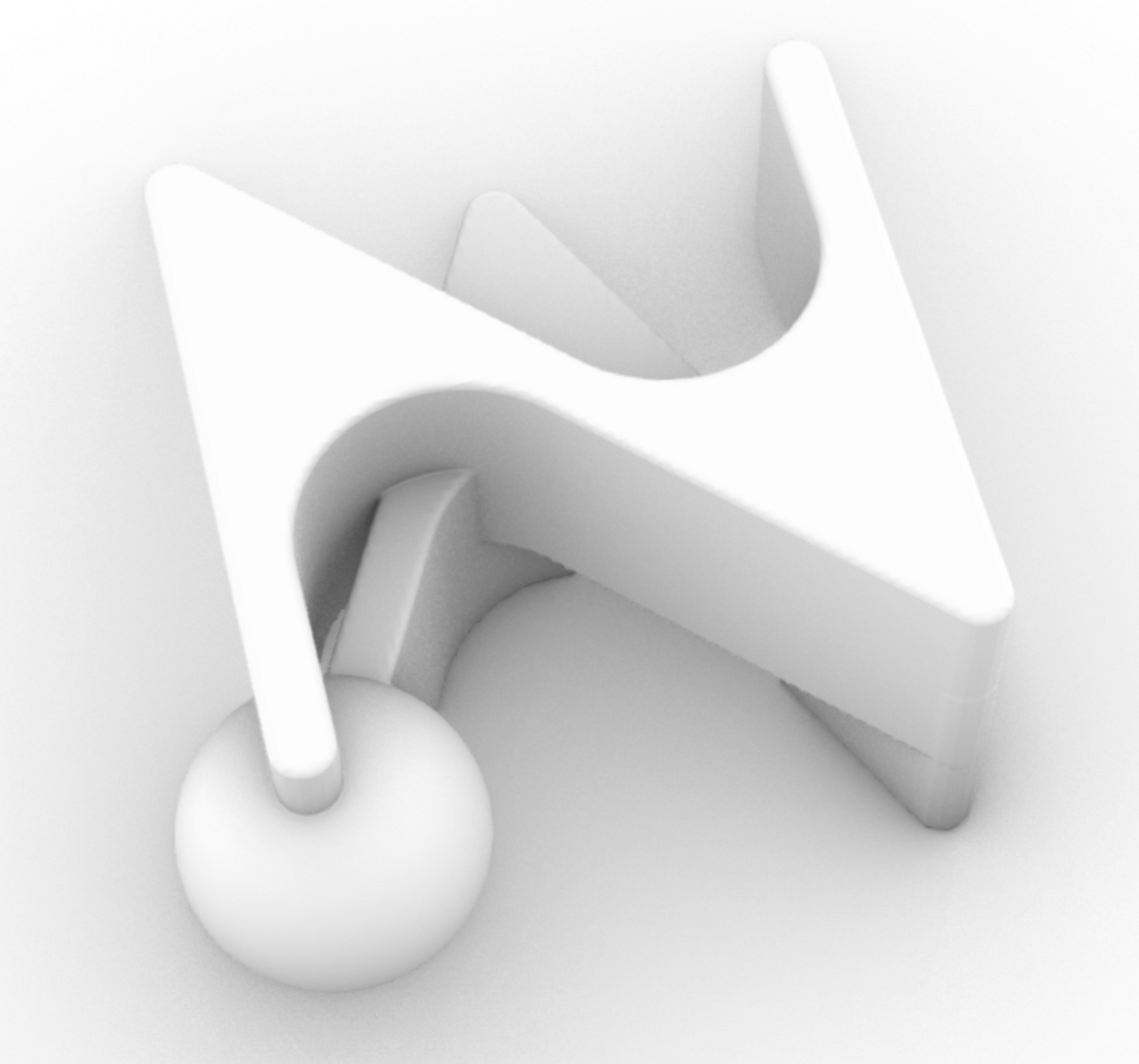
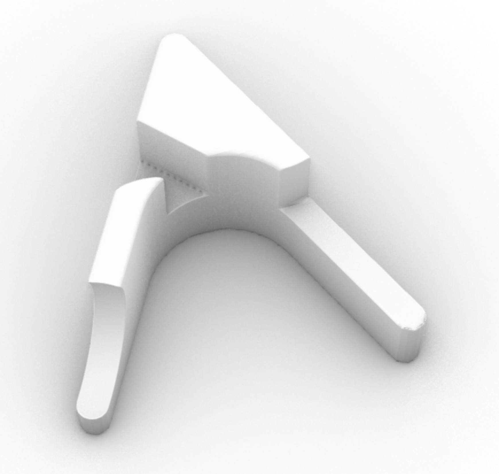
陰関数モデリングの利点として、ブーリアン演算(形状同士の足し算や引き算)も陰関数で表すことができ、演算が失敗しにくい点があります。
例えば、陰関数\(F_1<0,F_2<0\)により定義される2つの形状\(G_1,G_2\)があったときに、陰関数\(F=\min(F_1,F_2)<0\)で表される形状は\(G_1\)と\(G_2\)を足したもの、陰関数\(F=\max(F_1,-F_2)<0\)で表される形状は\(G_1\)から\(G_2\)を引いたものものとなります。
陰関数を用いたモデリング
波状の板
以下のように三角関数の和で陰関数を定義すれば、波状の板となります。
\(F(x,y,z)=|\cos (k_xx+\phi_x)+\cos (k_yy+\phi_y) +k_zz|-t<0\)
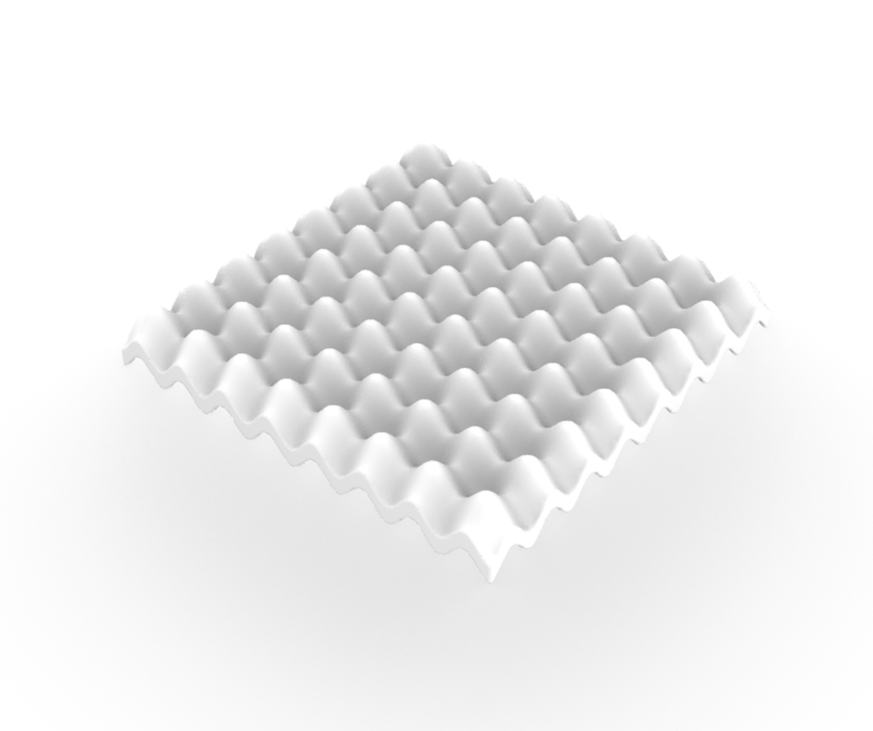
パラメータ\(k_x,k_y,k_z,\phi_x,\phi_y\)を連続的に変化させれば、形状が変化していく様子が見て取れます。
TPMS
\(z\)方向にも三角関数で変化する陰関数とすれば、TPMSの一種であるSchwarz Pに厚みを持たせた構造となります
\(\text{Schwarz P}:F(x,y,z)=|\cos x+\cos y+\cos z +s|-t<0\)
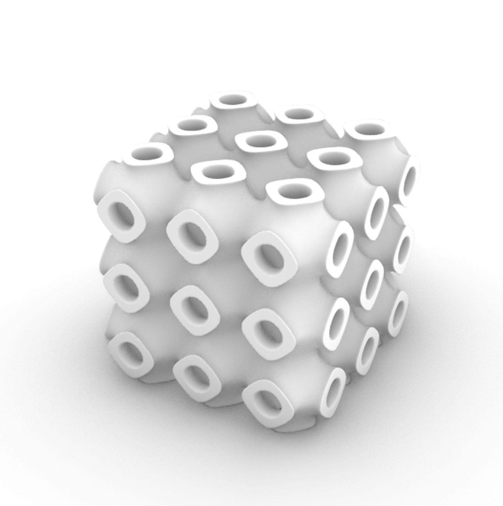
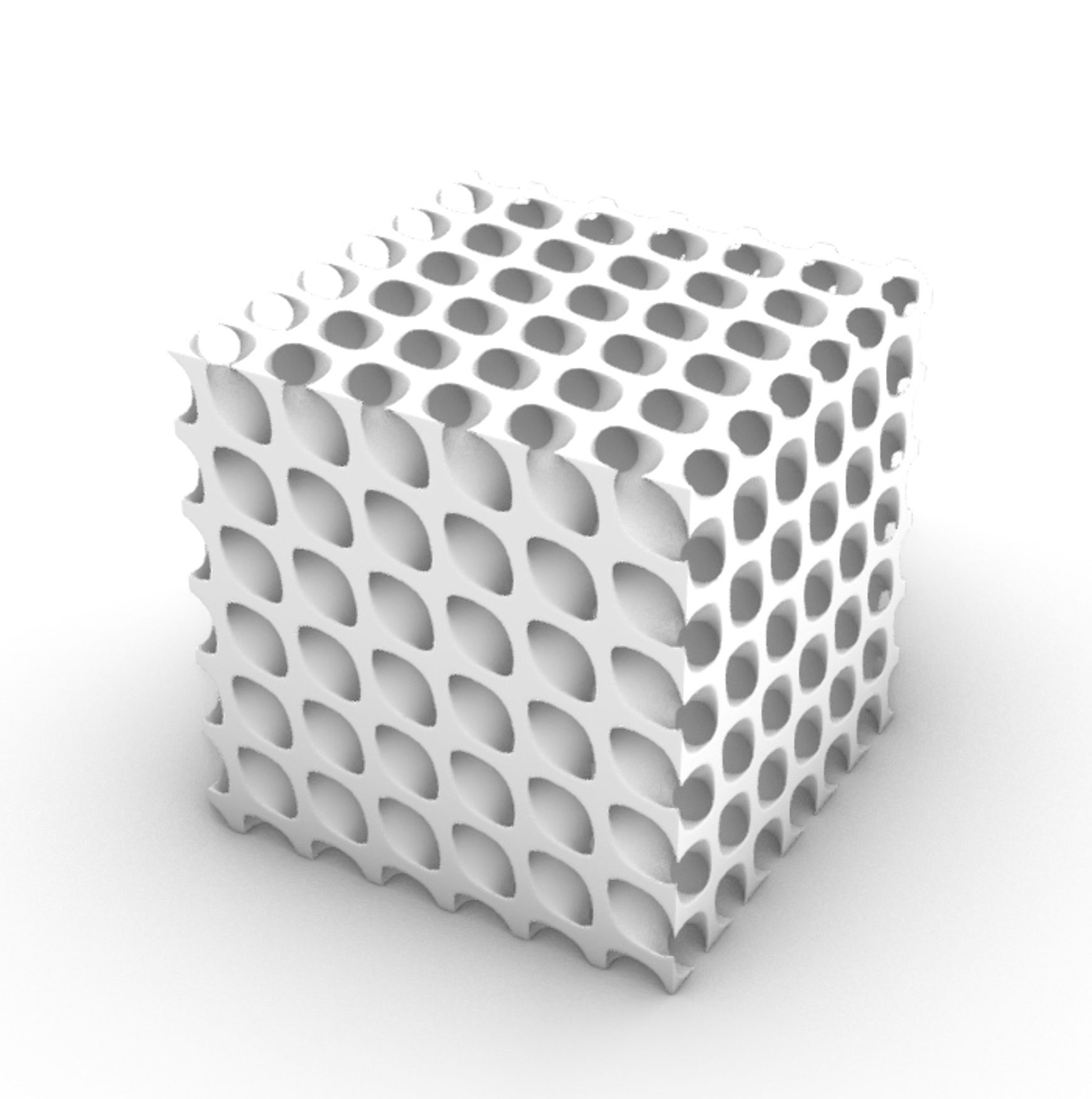
他にもよく陰関数モデリングの例としてGyroidやSchwarz Dがあげられますが、それぞれ厚みを持たせた陰関数表記と形状は以下のようになります。
\(\text{Gyroid}:F(x,y,z)=|\sin x\cos y+\sin y\cos z+\sin z\cos x +s|-t<0\)
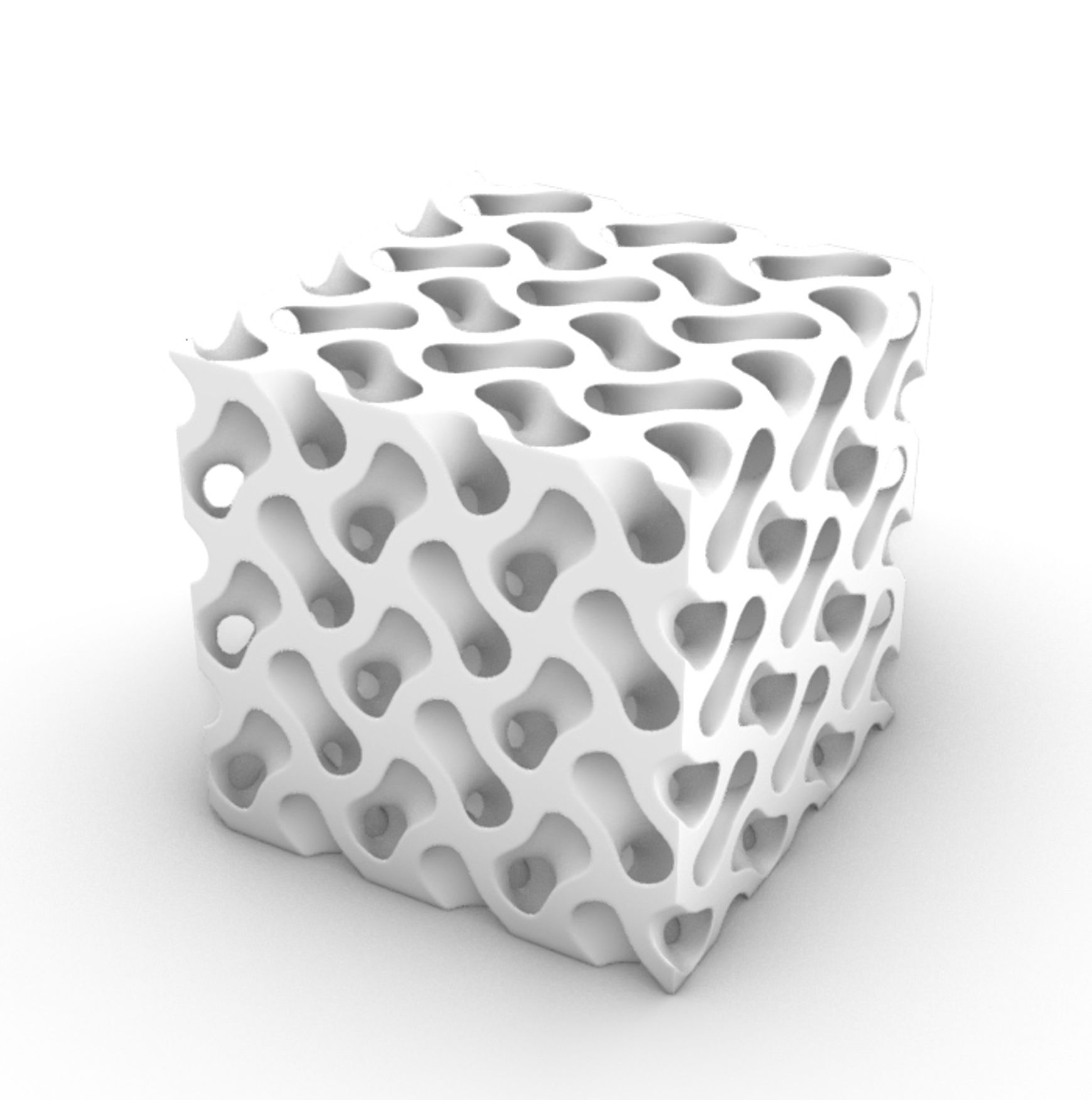
\(\text{Schwarz D}:F(x,y,z)=|\sin x\sin y\sin z+\sin x\cos y\cos z+\cos x\sin y\cos z+\cos x\cos y\sin z +s|-t<0\)
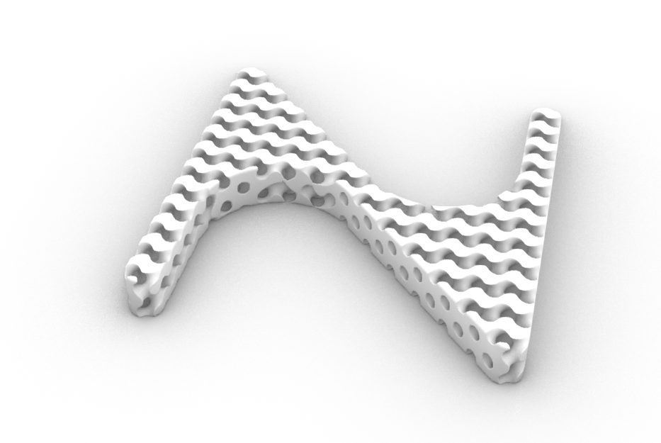
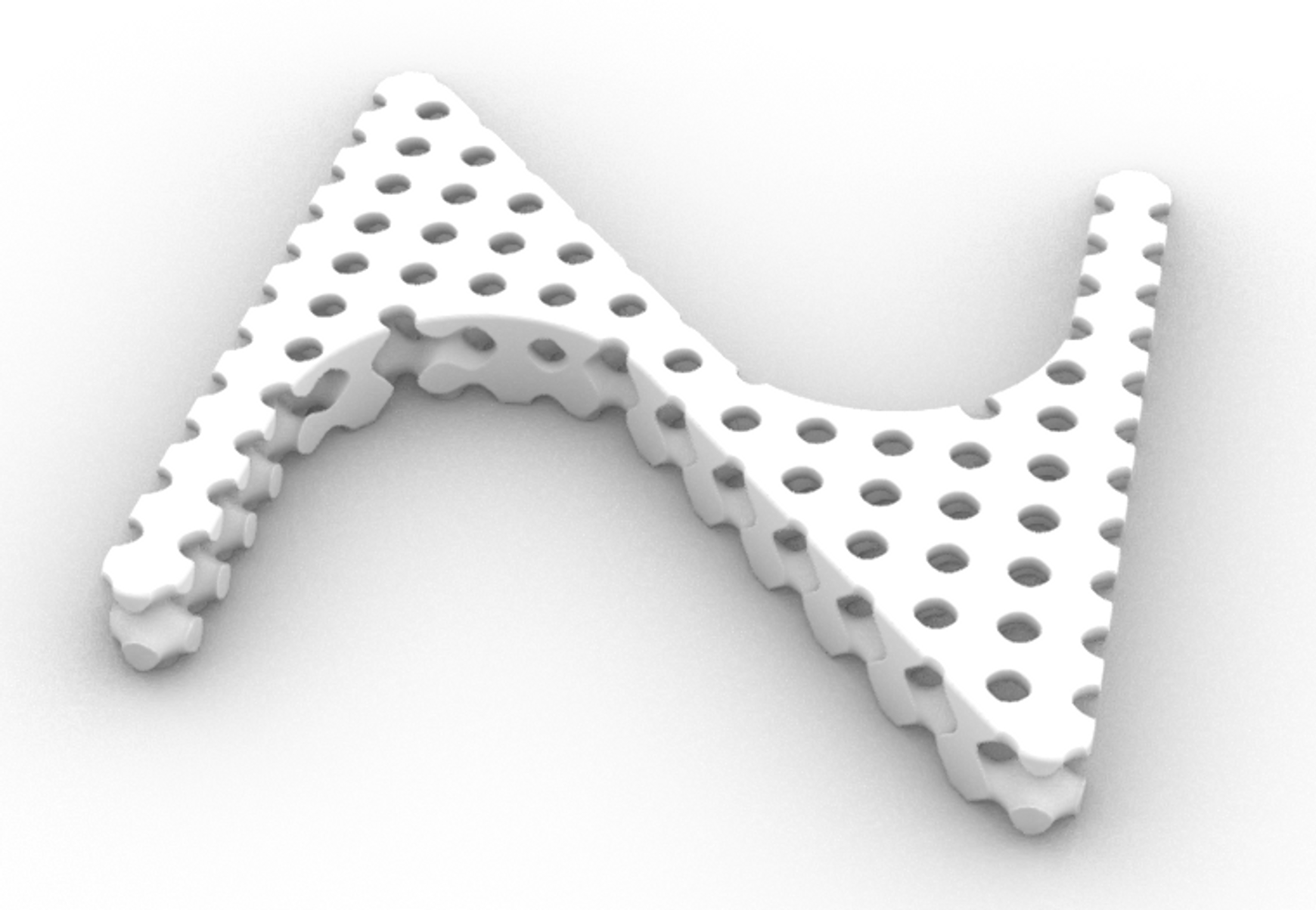
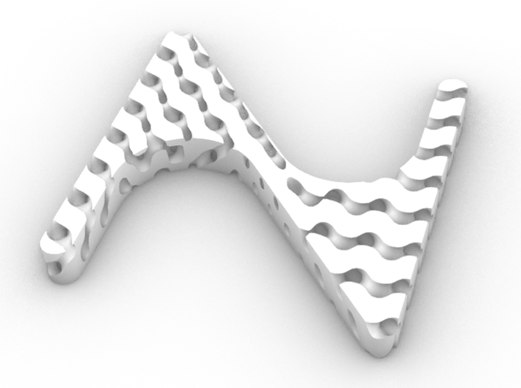
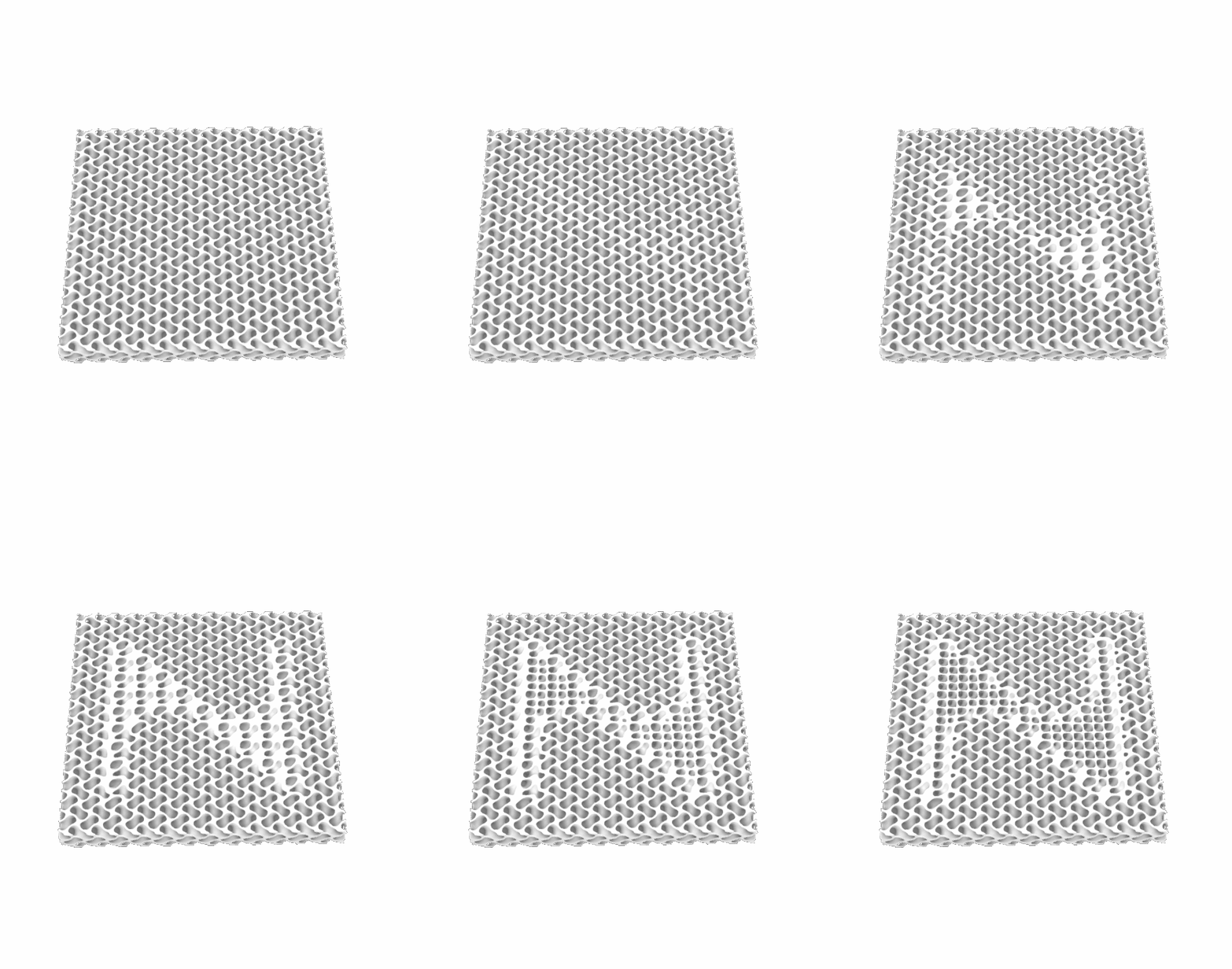
アイキャッチの画像はGyroidに厚みを持たせ、Nature ArchitectsのロゴNに割り当てたものです。
同様にSchwarz P, Dも容易に割り当てることができます。
TPMSの陰関数を拡張したモデリング
TPMSの陰関数を拡張していくつかモデリングをしていきます。
変化のスケールを変える
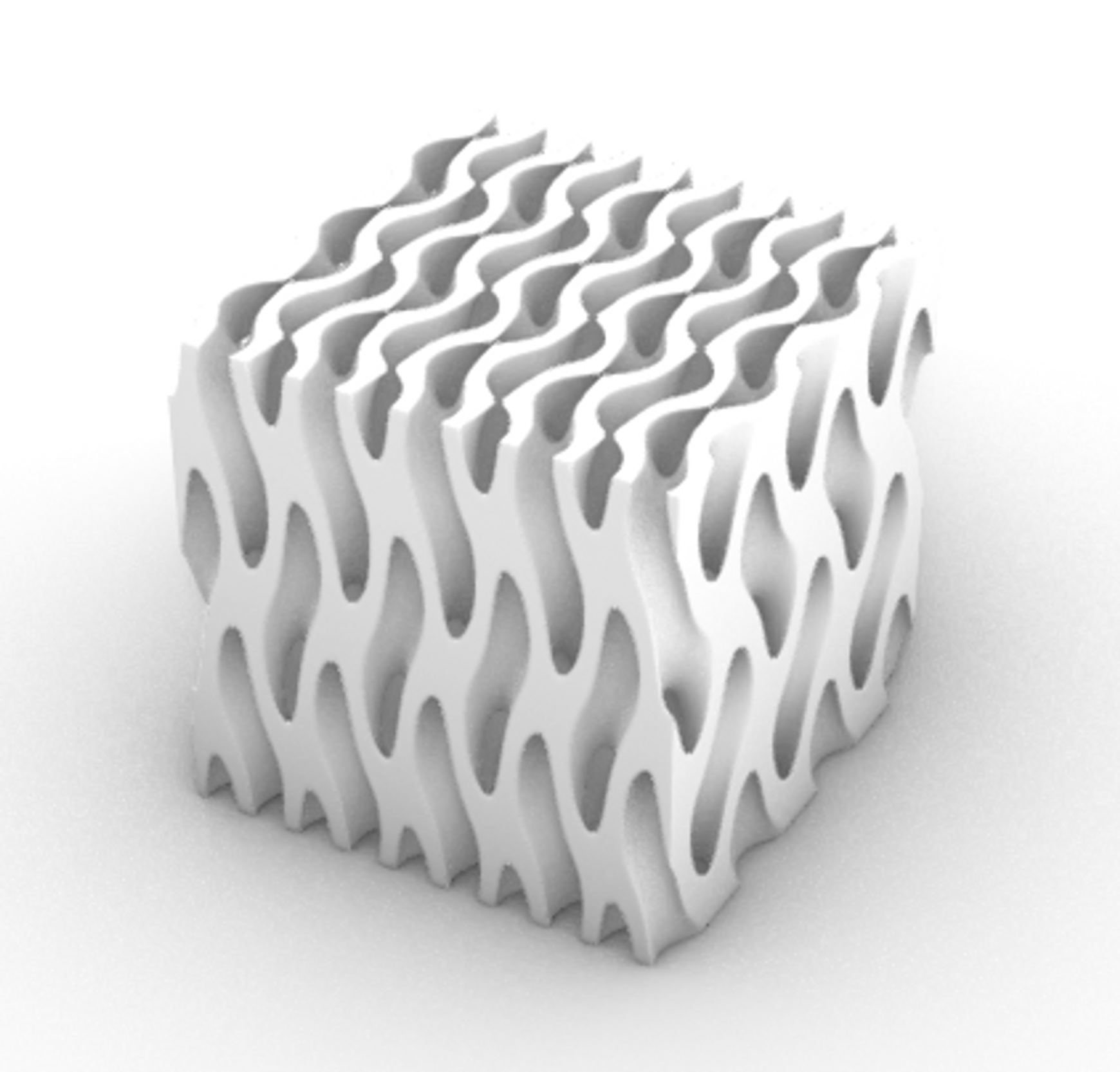
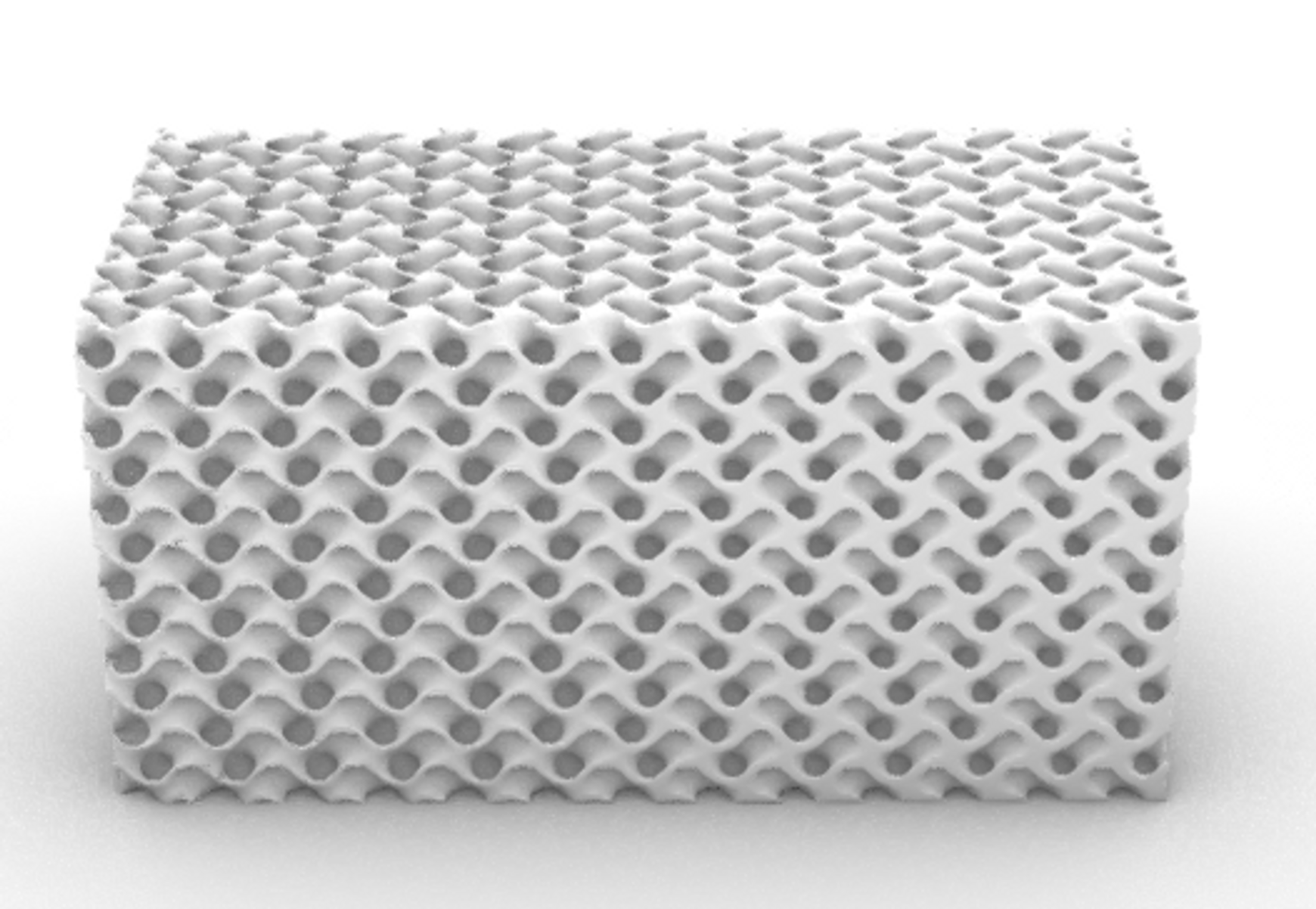
Gyroidの陰関数に、\(x,y,z\)方向の変化のスケールを決めるパラメータ\(k_x,k_y,k_z\)を導入し、\(k_x,k_y,k_z\)に異なる値を設定すれば各方向の周期を変えることができます。
\(F(x,y,z)=|\sin k_xx\cos k_yy+\sin k_yy\cos k_zz+\sin k_zz\cos k_xx +s|-t<0\)
厚みを連続的に変える
また、厚みのオフセットパラメータ\(s\)を変えると、厚みをつける位置を変えることができます。
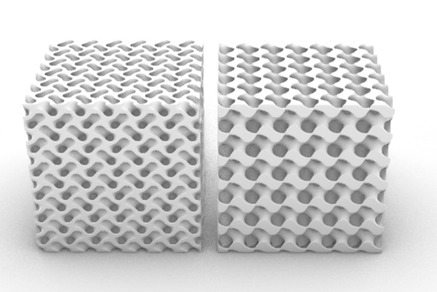
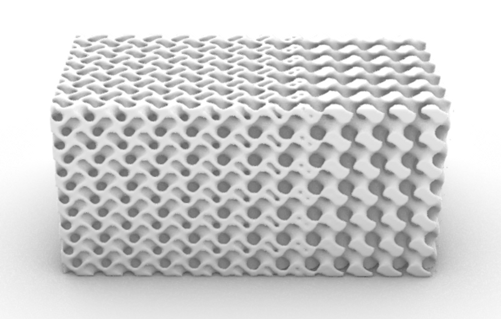
ここでパラメータ\(s\)を空間座標によって変わる関数にすると、厚みをつける位置を連続的に変えることができます。
\(F(x,y,z)=|\sin k_xx\cos k_yy+\sin k_yy\cos k_zz+\sin k_zz\cos k_xx +s(x,y,z)|-t<0\)
同様に厚みを決めるパラメータ\(t\)を関数とすれば、厚みを変化させることができます。
円筒座標・極座標でGyroidをつくる
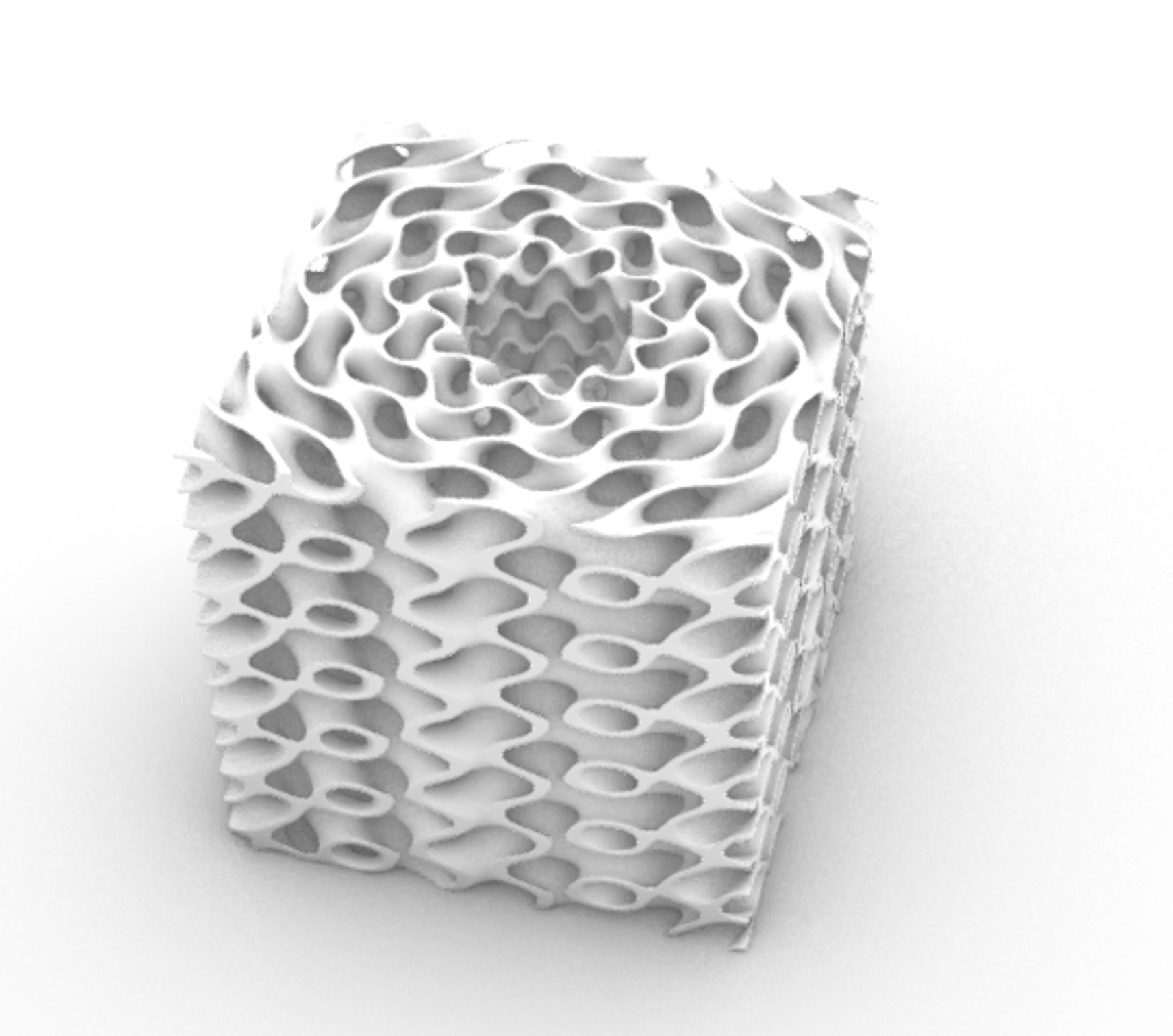
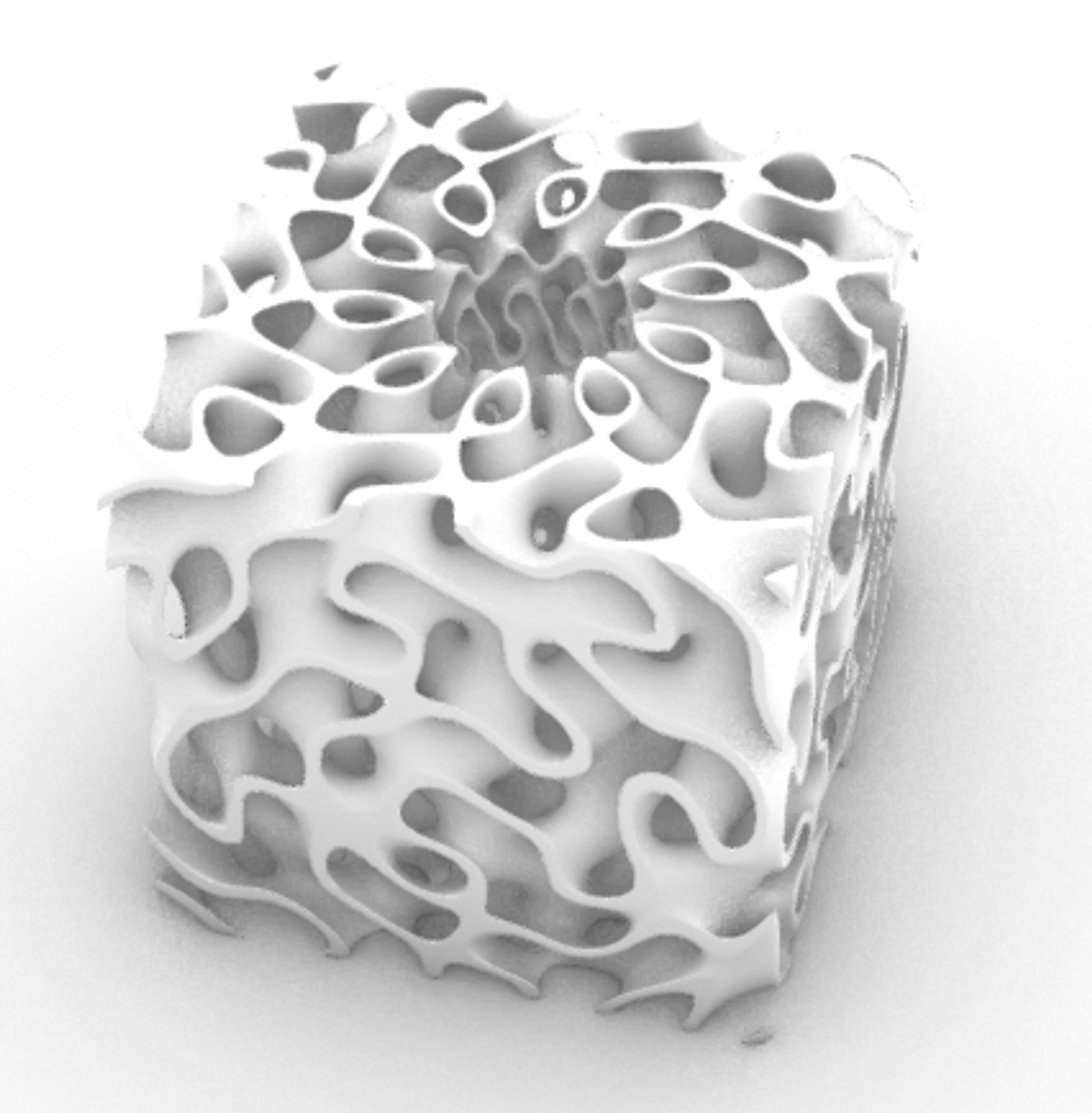
座標系を円筒座標・三次元極座標に変えてGyroidの陰関数を定義すれば、円筒状・球状にGyroidを割り当てることもできます。
\(F(r,\theta,z)=|\sin k_r r\cos n_{\theta}\theta+\sin n_{\theta}\theta\cos k_zz+\sin k_zz\cos k_rr +s|-t<0\)
\(F(r,\theta,\phi)=|\sin k_r r\cos n_{\theta}\theta+\sin n_{\theta}\theta\cos n_{\phi}\phi+\sin n_{\phi}\phi\cos k_rr +s|-t<0\)
異なるTPMSを補間する
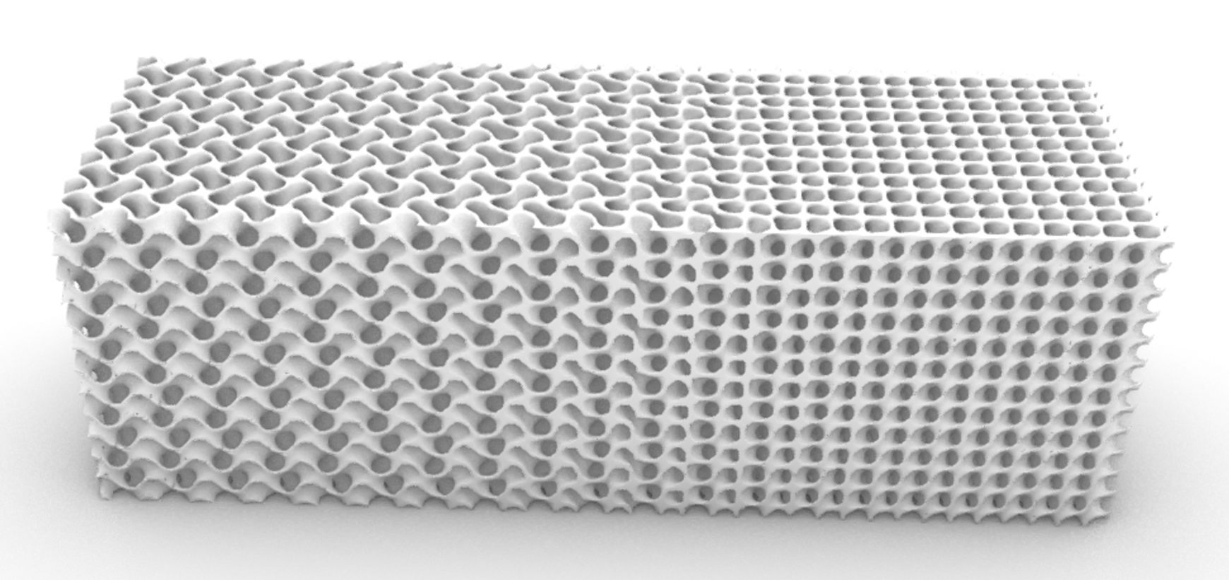
異なるTPMSの陰関数を足し合わせて新しい陰関数を作ることで、中間形状を作ることもできます。
\(\text{Gyroid}:F_G(x,y,z)=\sin k_xx\cos k_yy+\sin k_yy\cos k_zz+\sin k_zz\cos k_xx
\\
\text{Schwarz D}:F_D(x,y,z)=\sin k'_xx\sin k'_yy\sin k'_zz+\sin k'_xx\cos k'_yy\cos k'_zz+\cos k'_xx\sin k'_yy\cos k'_zz+\cos k'_xx\cos k'_zy\sin k'_zz
\\
F(x,y,z)=|aF_G(x,y,z)+(1-a)F_D(x,y,z)+s|-t<0\)
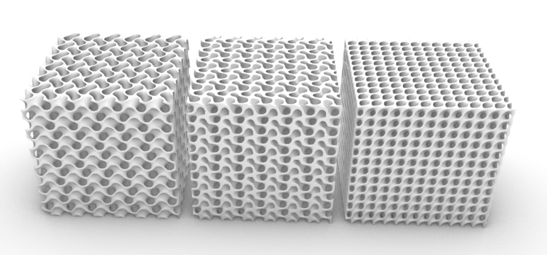
混合パラメータ\(a\)を空間座標によって変わる関数にすれば、GyroidからSchwarz Dに連続的に変化させることができます。
最後に
本章では陰関数モデリングの説明と、TPMSによるモデリングの実演をしてきました。
次章では、形状を引数とした陰関数によるモデリングについて解説します。
Introduction
This article will explain and demonstrate Implicit Modeling in the following two parts.
- Explanation of Implicit Modeling, modeling by TPMS (Triply Periodic Minimal Surface)
- Implicit modeling with geometry as an argument
The modeling is mainly done using the Rhinoceros-Grasshopper plug-in Jellyfish.
In Chapter 1, we will explain implicit modeling and perform various modeling with TPMS.
What is Implicit Modeling?
A function in solved form with respect to one of the variables, such as \(y = f(x)\), is called an explicit function. On the other hand, a function that is not written in solved form, such as \(F(x, y) = 0\), is called an implicit function. Implicit modeling is a method of modeling geometry in terms of implicit functions.
For example, when modeling a circle, the implicit function is defined as follows
\(F(x,y)=x^2+y^2-R^2\)
Modeling is performed by defining regions with equality or inequality based on this implicit function.
For example, in the above implicit function, assuming \(R=5\) and generating a shape in the region \(F(x,y)=0\), the following circle is generated in the \(xy\) plane. (For convenience of visualization, the circle is given a thickness)
If \(F(x,y)\leq 0\), the interior is a filled circle.
If \(F(x,y,z)=x^2+y^2+z^2-R^2< 0\), then it is a sphere.
One of the advantages of implicit modeling is that boolean operations (addition and subtraction of shapes) can also be represented by implicit functions, making it difficult for operations to fail.
For example, if there are two shapes \(G_1,G_2\) defined by the implicit function \(F_1<0,F_2<0\), the shape represented by the implicit function \(F=\min(F_1,F_2)<0\) is the sum of \(G_1\) and \(G_2\), while the shape represented by the implicit function \(F=\max(F_1,-F_2)<0\) is \(G_1\) minus \(G_2\).
Modeling with implicit functions
Corrugated plate
If we define the implicit function by the sum of the trigonometric functions as follows, we get a Corrugated plate.
\(F(x,y,z)=|\cos (k_xx+\phi_x)+\cos (k_yy+\phi_y) +k_zz|-t<0\)
If you continuously change the parameters \(k_x,k_y,k_z,\phi_x,\phi_y\), you can see how the shape changes.
TPMS
If we make it an implicit function that also varies trigonometrically in the `\(z\) direction, the structure is a kind of TPMS, Schwarz P with thickness
\(\text{Schwarz P}:F(x,y,z)=|\cos x+\cos y+\cos z +s|-t<0\)
Other common examples of implicit modeling are Gyroid and Schwarz D. The implicit notation and geometry of each with thickness are shown below.
\(\text{Gyroid}:F(x,y,z)=|\sin x\cos y+\sin y\cos z+\sin z\cos x +s|-t<0\)
\(\text{Schwarz D}:F(x,y,z)=|\sin x\sin y\sin z+\sin x\cos y\cos z+\cos x\sin y\cos z+\cos x\cos y\sin z +s|-t<0\)
The eye-catching image is a thicker version of Gyroid, assigned to the Nature Architects logo N.
Similarly, Schwarz P, D can be easily assigned.
Modeling with extended TPMS implicit functions
We will do some modeling by extending the implicit functions of TPMS.
Changing the Scale of Change
Introducing the parameter \(k_x,k_y,k_z\), which determines the scale of change in the \(x,y,z\) direction, to Gyroid's implicit function, and setting different values for \(k_x,k_y,k_z\) will change the period in each direction.
\(F(x,y,z)=|\sin k_xx\cos k_yy+\sin k_yy\cos k_zz+\sin k_zz\cos k_xx +s|-t<0\)
Continuously varying thickness
You can also change the position where the thickness is applied by changing the thickness offset parameter \(s\).
If the parameter \(s\) is a function that varies with spatial coordinates, the position of the thickness can be changed continuously.
\(F(x,y,z)=|\sin k_xx\cos k_yy+\sin k_yy\cos k_zz+\sin k_zz\cos k_xx +s(x,y,z)|-t<0\)
Similarly, if the parameter \(t\), which determines the thickness, is a function, the thickness can be varied.
Create Gyroid with cylindrical and polar coordinates
You can also assign Gyroid to cylindrical or spherical shapes by changing the coordinate system to cylindrical or three-dimensional polar coordinates and defining the implicit function of Gyroid.
\(F(r,\theta,z)=|\sin k_r r\cos n_{\theta}\theta+\sin n_{\theta}\theta\cos k_zz+\sin k_zz\cos k_rr +s|-t<0\)
\(F(r,\theta,\phi)=|\sin k_r r\cos n_{\theta}\theta+\sin n_{\theta}\theta\cos n_{\phi}\phi+\sin n_{\phi}\phi\cos k_rr +s|-t<0\)
Complement different TPMS
Intermediate shapes can also be created by adding together different TPMS implicit functions to create a new implicit function.
\(\text{Gyroid}:F_G(x,y,z)=\sin k_xx\cos k_yy+\sin k_yy\cos k_zz+\sin k_zz\cos k_xx
\\
\text{Schwarz D}:F_D(x,y,z)=\sin k'_xx\sin k'_yy\sin k'_zz+\sin k'_xx\cos k'_yy\cos k'_zz+\cos k'_xx\sin k'_yy\cos k'_zz+\cos k'_xx\cos k'_zy\sin k'_zz
\\
F(x,y,z)=|aF_G(x,y,z)+(1-a)F_D(x,y,z)+s|-t<0\)
If the mixing parameter \(a\) is a function that varies with spatial coordinates, it can be varied continuously from Gyroid to Schwarz D.
Conclusion
In this chapter, we have explained implicit function modeling and demonstrated modeling with TPMS.
In the next chapter, we will discuss modeling by implicit functions with shape as an argument.
